Approaching Classification With Neural Networks

This article was published as a part of the Data Science Blogathon.

Introduction on Classification

Classification is one of the basic tasks that a machine can be trained to perform. This can include classifying whether it will rain or not today using the weather data, determining the expression of the person based on the facial image, or the sentiment of the review based on text etc. Classification is extensively applied in various applications thus making it one of the most fundamental tasks under supervised machine learning.

There are various algorithms used to perform classification based on the type of dataset being considered. This ranges from tree-based classifiers like Random Forests and decision trees, to gradient boosted algorithms like XGboost or neural networks based classifiers. In this blog, let’s explore how to use neural networks to build custom classifiers for a tabular dataset. The advantage of using neural networks is that we can easily detect and learn unknown patterns present in the data.

But before we start with the classification let’s get started…

About the Dataset

The dataset we are using to train our model is the Iris Dataset. This dataset consists of 150 samples belonging to 3 species of Iris flower i.e. Iris Setosa, Iris Versicolour and Iris Virginica. This is a multi-variate dataset i.e. there are 4 features provided for each sample i.e. sepal length, sepal width, petal length and petal width. We need to use these 4 features and classify the type of iris species. Thus a multi-class classification model is used to train on this dataset. More information about this dataset can be found here.

Getting Started with Classification

Let’s get started by first importing required libraries,

import os
import pandas as pd
import matplotlib.pyplot as plt
import numpy as np
import tensorflow as tf
from tensorflow.keras import Sequential
from tensorflow.keras import layers
from tensorflow.keras import models
from tensorflow.keras import optimizers
from tensorflow.keras import losses
from tensorflow.keras import metrics
from sklearn.preprocessing import StandardScaler
from sklearn.model_selection import train_test_split
from sklearn.metrics import classification_report, accuracy_score
from tensorflow import keras
from sklearn.preprocessing import LabelEncoder

Check the version of TensorFlow installed by following,

print(tf.__version__)

Next, we need to download and extract the dataset from here. Then move it to the location of notebook/script or copy the location of the dataset. Now read the CSV file from that location,

file_path = 'iris_dataset.csv'
df = pd.read_csv(file_path)
df.head()

We can see that our dataset has 4 input features and 1 target variable. The target variable consists of 3 classes i.e. ‘Iris-setosa’, ‘Iris-versicolor’ and ‘Iris-verginica’. Now let’s further prepare our dataset for model training.

Data Preparation

First, let’s check if our dataset consists of any null values.

print(df.isnull().sum())

There are no null values. Therefore we can continue to separate the inputs and targets.

X = df.drop('target', axis=1)
y = df['target']

Since now we have separated the input features (X) and target labels (y), let’s split the dataset into training and validation sets. For this purpose let’s use Scikit-Learn’s train_test_split method to split our dataset.

X_train, X_test, y_train, y_test = train_test_split(X, 
                                                    y, 
                                                    test_size=0.2, 
                                                    random_state=42)

print("The length of training dataset: ", len(X_train))
print("The length of validation dataset: ", len(X_test))

In the above code, we have split the dataset such that the validation data contains 20% of the randomly selected samples from the whole dataset. Let’s now further do some processing before we create the model.

Data Processing

Since we have the data split ready, let’s now do some basic processing like feature scaling and encoding labels. The input features contain attributes of petal and sepal i.e. length and width in centimetres. Therefore these features are numerical that need to be normalized i.e. transform the data such that the mean is 0 and the standard deviation is 1.

Let’s use Scikit-learn’s StandardScalar module to do the same.

features_encoder = StandardScaler()
features_encoder.fit(X_train)
########################################################
X_train = features_encoder.transform(X_train)
X_test = features_encoder.transform(X_test)

Now we should encode the categorical target labels. This is because our model won’t be able to understand if the categories are represented in strings. Therefore let’s encode the labels using Scikit-learn’s LabelEncoder module.

label_encoder = LabelEncoder()
label_encoder.fit(y_train)
########################################################
y_train = label_encoder.transform(y_train).reshape(-1, 1)
y_test = label_encoder.transform(y_test).reshape(-1, 1)

Now let’s check the shapes of the datasets,

print(X_train.shape)
print(X_test.shape)
print(y_train.shape)
print(y_test.shape)

Great! Now we are ready to define and train our model.

Creating Model

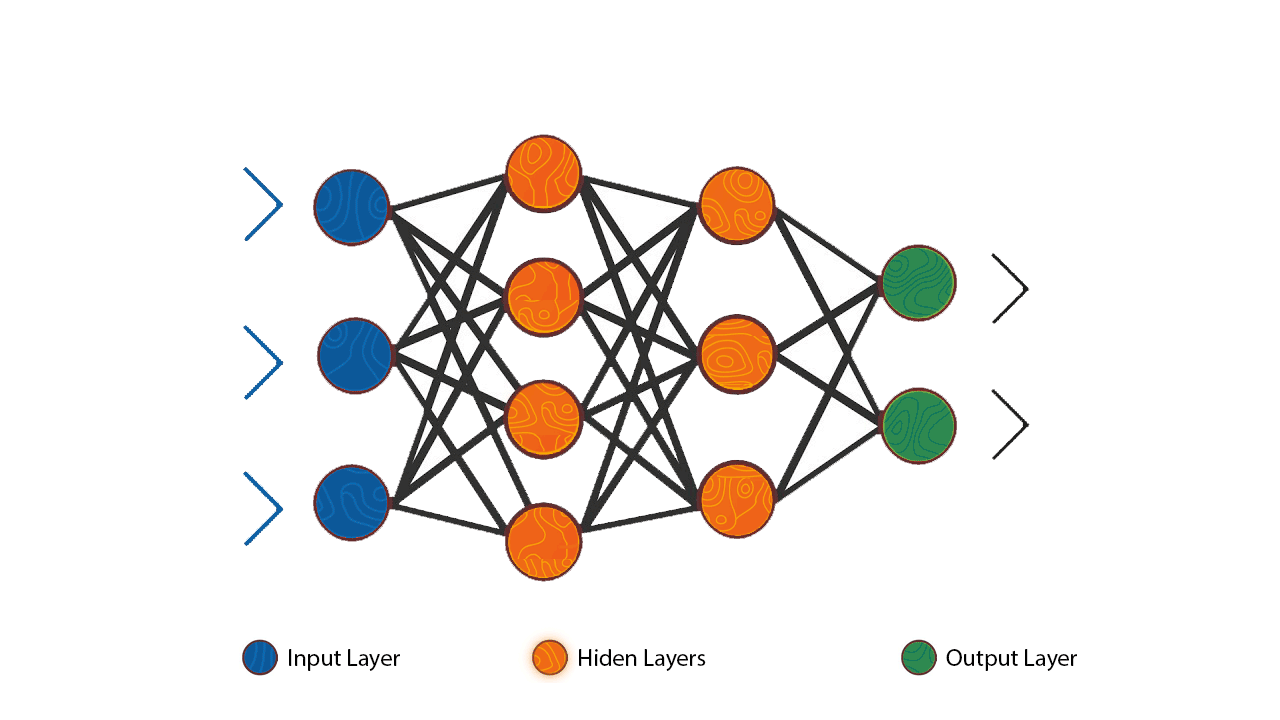
Let’s define the model for classification using the Keras Sequential API. We can stack the required layers and define the model architecture. For this model, let’s define Dense layers to define the input, output and intermediate layers.

model = Sequential([
    layers.Dense(8, activation="relu", input_shape=(4,)),
    layers.Dense(16, activation="relu"),
    layers.Dense(32, activation="relu"),
    layers.Dense(3, activation="softmax")
])

In the above model, we have defined 4 Dense layers. The output layer consists of 3 neurons i.e. equal to the number of output labels present. We are using the softmax activation function at the final layer because it enables the model to provide probabilities for each of the labels. The output label that has the highest probability is the output prediction determined by the model. In other layers, we have used the relu activation function.

Now let’s compile the model by defining the loss function, optimizer and metrics.

model.compile(optimizer=optimizers.SGD(),
              loss=losses.SparseCategoricalCrossentropy(),
              metrics=metrics.SparseCategoricalAccuracy())

According to the above code, we have used SGD or Stochastic Gradient Descent as the optimizer with a default learning rate of 0.01. The SparseCategoricalCrossEntropy loss function is used. We are using SparseCategoricalCrossEntropy rather than CategoricalCrossEntropy loss function because our outputs categories are in the integer format. CategoricalCrossEntropy would be a good choice when the categories are one-hot encoded. Finally, we are using SparseCategoricalAccuracy as the metric that is tracked.

Now let’s train the model…

Model Training and Evaluation

Now let’s train our model using the processed training data for 200 epochs and provide the test dataset for validation.

history = model.fit(x=X_train,
          y=y_train,
          epochs=200,
          validation_data=(X_test, y_test),
          verbose=0)

Now we have trained our model using the training dataset. Before evaluation let’s check the summary of the model we have defined.

# Check model summary
model.summary()

Now let’s evaluate the model on the testing dataset.

# Perform model evaluation on the test dataset
model.evaluate(X_test, y_test)

That’s great results… Now let’s define some helper functions to plot the accuracy and loss plots.

# Plot history
# Function to plot loss
def plot_loss(history):
    plt.plot(history.history['loss'], label='loss')
    plt.plot(history.history['val_loss'], label='val_loss')
    plt.ylim([0,10])
    plt.xlabel('Epoch')
    plt.ylabel('Error (Loss)')
    plt.legend()
    plt.grid(True)
########################################################
# Function to plot accuracy
def plot_accuracy(history):
    plt.plot(history.history['sparse_categorical_accuracy'], label='accuracy')
    plt.plot(history.history['val_sparse_categorical_accuracy'], label='val_accuracy')
    plt.ylim([0, 1])
    plt.xlabel('Epoch')
    plt.ylabel('Accuracy')
    plt.legend()
    plt.grid(True)

Now let’s pass the model training history and check the model performance on the dataset.

plot_loss(history)
plot_accuracy(history)

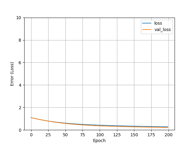
We can see from the graphs below that the model has learnt over time to classify different species almost accurately.

Save and Load Model

Since we have the trained model,  we can export it for further use cases, deploy it in applications, or continue the training from left off. We can do this by using the save method and exporting the model in H5 format.

# Save the model
model.save("trained_classifier_model.h5")

We can load the saved model checkpoint by using the load_model method.

# Load the saved model and perform classification
loaded_model = models.load_model('trained_classifier_model.h5')

Now let’s try to find predictions from the loaded model. Since the model contains softmax as the output activation function, we need to use the np.argmax() method to pick the class with the highest probability.

# The results the model returns are softmax outputs i.e. the probabilities of each class.
results = loaded_model.predict(X_test)
preds = np.argmax(results, axis=1)

Now we can evaluate the predictions by using metric functions.

# Predictions
print(accuracy_score(y_test, preds))
print(classification_report(y_test, preds))

Awesome! Our results match the previous ones.

Conclusion on Classification

Till now we have trained a deep neural network using TensorFlow to perform basic classification tasks using tabular data. By using the above method, we can train classifier models on any tabular dataset with any number of input features. By leveraging the different types of layers available in Keras, we can optimize and have more control over the model training, thus improving the metric performance. It is recommended to try replicating the above procedure on other datasets and experiment by changing different hyperparameters like learning rate, the number of layers, optimizers etc until we get desirable model performance.