Big Data with Spark and Scala
This article was published as a part of the Data Science Blogathon.
Introduction
Big Data is a new term that is used widely in every section of society. Be it in agriculture, research, manufacturing, you name it and there this technology is widely used. Big Data is a field that treats ways to analyze, systematically extract information from, or otherwise, deal with datasets that are too large or complex to be dealt with by traditional data processing applications.
Big Data is often characterized by:-
a) Volume:- Volume means a huge and enormous amount of data that needs to be processed.
b) Velocity:- The speed with which data arrives like real-time processing.
c) Veracity:- Veracity means the quality of data (that actually needs to be great to use for generating analysis reports etc.)
d) Variety:- It means the different types of data like
* Structured Data:- Data in table format.
* Unstructured Data:- Data not in table format
* Semi-Structured Data:- Mix of both structured and unstructured data.
To work with large bytes of data first we need to store or dump the data somewhere. Thus, the solution to this is HDFS(Hadoop Distributed File System).
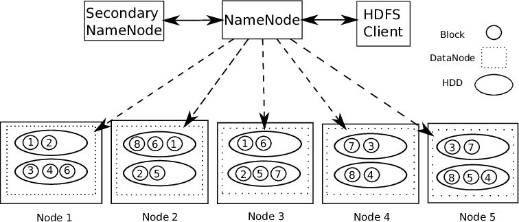
Hadoop supports Master-Slave architecture. It is a distributed type of system where the parallel processing of data is done. Hadoop consists of 1 master and multiple slaves.
Rule of Name Node:- For every block of data that is stored, 2 copies are present. One in different data nodes and 2nd copy in another data node. Thus, solving the problem of fault tolerance.
Name node contains the following information:-
1) Metadata information of the files stored in the data nodes. Metadata consists of 2 files – FsImage and EditLogs. FsImage consists of the complete state of the file system since the start of the Name Node. EditLogs contains recent modifications that are made to the file system.
2) location of the file block stored in the data node.
3) Size of files.
The data node contains the actual data.
Thus, HDFS supports data integrity. The data that is stored is checked whether it is correct or not by checking data against its checksum. If any faults are detected, it gets reported to the Name Node. So, it creates additional copies of the same data and deletes the corrupted copies.
HDFS consists of Secondary Name Node which works concurrently with the primary Name Node as helper daemon. It is not a backup Name Node. It reads constantly all file systems and metadata from RAM of Name Node to hard disk. It is responsible for combining EditLogs with FSImage from Name Node.
Thus, HDFS is like a data warehouse where we can dump any kind of data. Processing these data requires Hadoop tools like Hive( for handling structured data), HBase(for handling unstructured data), etc. Hadoop supports the “Write once Ready Many” concept.
So, Let’s take an example and understand how we can process a humungous amount of data and perform many transformations using Scala Language.
A) Setting up Eclipse IDE with Scala setup.
Link to download eclipse IDE – https://www.eclipse.org/downloads/
You need to download the Eclipse IDE considering your computer requirements. On starting the eclipse IDE you will see this type of screen.
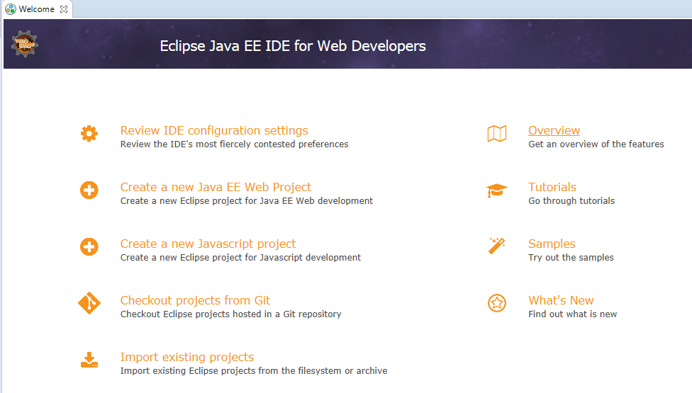
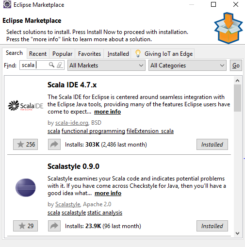
Go to Help -> Eclipse Marketplace -> Search -> Scala-Ide -> Install
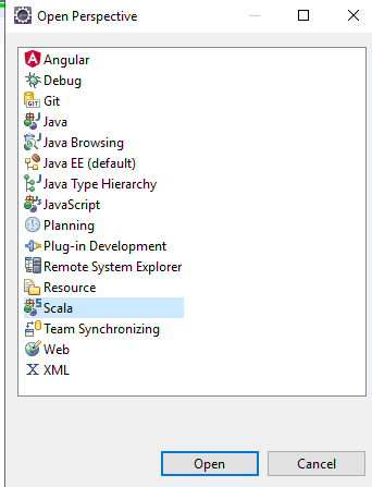
After that on Eclipse IDE – select Open Perspective -> Scala, you will get all the scala components in the ide to use.
Create a new project in eclipse and update the pom file with the following steps –https://medium.com/@manojkumardhakad/how-to-create-maven-project-for-spark-and-scala-in-scala-ide-1a97ac003883
Change the scala library version by right-clicking on Project -> Build Path -> Configure Build Path.
Update the project by right-clicking on Project -> Maven -> Update Maven Project -> Force Update of Snapshots/Releases. Thus, the pom file gets saved and all required dependencies get downloaded for the project.
After that download the spark version with Hadoop winutils placed in the bin path. Follow this path to get the setup done – https://stackoverflow.com/questions/25481325/how-to-set-up-spark-on-windows
B) Creating Spark Session – 2 types.
Spark Session is the entry point or the start to create RDD’S, Dataframe, Datasets. To create any spark application firstly we need a spark session.
Spark Session can be of 2 types:-
a) Normal Spark session:-
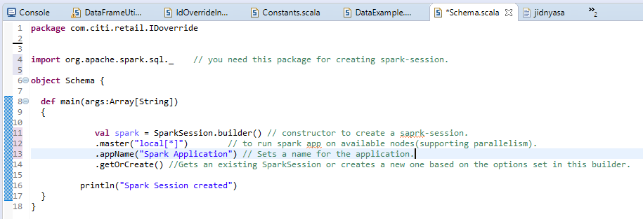
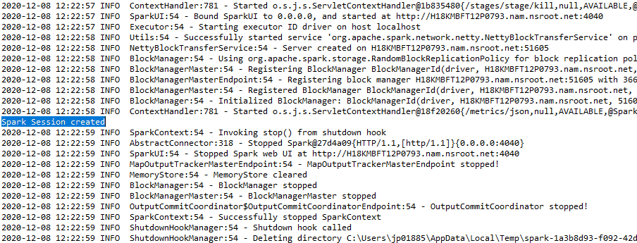
The output will be shown as:-
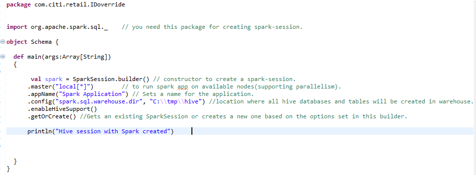
b) Spark Session for Hive Environment:-
For creating a hive environment in scale, we need the same spark-session with one extra line added. enableHiveSupport() – enables Hive support, including connectivity to persistent Hive metastore, support for hive serdes, and Hive user-defined functions.
C) RDD(Resilient Distributed Dataset) Creation and Transforming RDD to DataFrame:-
So after the 1st step of creating Spark-Session, we are free to create RDD’s, Datasets, or DataFrames. These are the data-structures in which we can store large enormous amounts of data.
Resilient:- means fault-tolerant so they can re-compute missing or damaged partitions due to node failures.
Distributed:- means data is distributed across multiple nodes(power of parallelism).
Datasets:- Data that can be loaded externally and that can be of any form i.e. JSON, CSV, or text-file.
Features of RDD’s includes:-
a) In-memory computation:- After performing transformations to data, the results are stored in RAM instead of a disk. Thus, large datasets cannot be used by RDD. The solution to this is instead of using RDD’s use of DataFrame/Dataset is considered.
b) Lazy Evaluations:- It means the actions of the transformations performed are evaluated only when the value is needed.
.jpg)
c) Fault Tolerance:- Spark RDD’s are fault-tolerant as they track data lineage information to rebuild lost data automatically on failure.
d) Immutability:- Immutable(Non-changeable) data is always safe to share across multiple processes. We can recreate the RDD at any time.
e) Partitioning:- Means dividing the data, thus each partition can be executed by different nodes thus processing of data becomes faster.
f) Persistence:- Users can choose which RDD’s they need to use and choose a storage strategy for them.
g) Coarse-Grained Operations:- It means that when data is partitioned across different clusters for different operations we can apply transformations once for the entire cluster and not for different partitions separately.
D) Dataframe usage and Performing Transformations:-
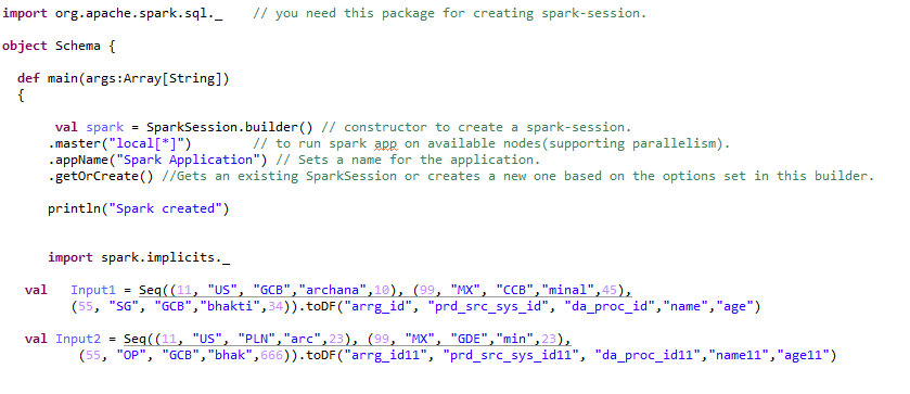
When converting RDD’s into data frames you need to add import spark.implicits._ after the spark session.
Dataframe can be created in many ways. Let’s see the different transformations that can be applied to the data frame.
Step 1:- Creating data frame:-
Step2:- Performing different types of transformations to a data frame:-
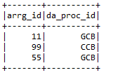
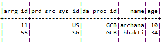
a) Select:- It selects the required columns of the data frame which the user requires.
Input1.select(“arrg_id”, “da_proc_id”).show()
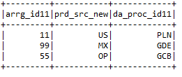
b) selectExpr:- It selects the required columns and also renames the columns as well.
Input2.selectExpr(“arrg_id11”,”prd_src_sys_id11 as prd_src_new “,”da_proc_id11”).show()
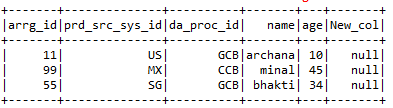
c) withColumn:- withColumns helps to add a new column with the particular value the user wants in the selected data frame.
Input1.withColumn(“New_col”,lit(null))
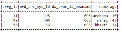
d) withColumnRenamed:- It renames the columns of the particular dataframe which the user requires.
Input1.withColumnRenamed(“da_proc_id”, “da_proc_id_newname”)
e) drop:- Drops the columns that the user doesn’t want.
Input2.drop(“arrg_id11″,”prd_src_sys_id11″,”da_proc_id11”)
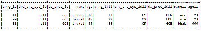
f) Join:- Joins 2 data frames together with joining keys of both data frames.
Input1.join(Input2, Input1.col(“arrg_id”) === Input2.col(“arrg_id11″),”right”)
.withColumn(“prd_src_sys_id”, lit(null))
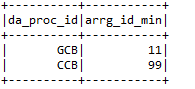
g) Aggregate Functions:- Some of the aggregate functions include
* Count:- It gives the count of a particular column or the count of the data frame as a whole.
println(Input1.count())

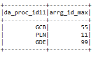
* Max:- It gives the maximum value of the column according to a particular condition.
input2.groupBy(“da_proc_id”).max(“arrg_id”).withColumnRenamed(“max(arrg_id)”,
“arrg_id_max”)
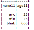
* Min:- It gives a minimum value from the data frame column.
h) filter:- It filters out the columns of a data frame by executing a particular condition.
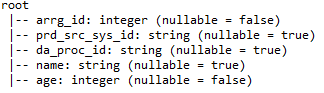
i) printSchema:- It gives the details such as column names, data-types of columns, and whether the columns can be nullable or not.
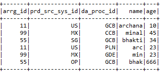
j) Union:- It combines the values from 2 data frames provided that the column names of both data frames are the same.
E) Hive:-
Hive is one of the most used databases in Big Data. It is a kind of relational database where data is stored in tabular format. The default database of the hive is the derby. Hive processes structured and semi-structured data. Incase of unstructured data, first create a table in the hive and load the data into the table thus making it structured. Hive supports all primitive datatypes of SQL.
Hive supports 2 kinds of tables:-
a) Managed Tables:- It is the default table in Hive. When the user creates a table in Hive without specifying it as external, then by default, an internal table gets created in a specific location in HDFS.
By default, an internal table will be created in a folder path similar to /user/hive/warehouse directory of HDFS. We can override the default location by the location property during table creation.
If we drop the managed table or partition, the table data, and the metadata associated with that table will be deleted from the HDFS.
b) External table:- External tables are stored outside the warehouse directory. They can access data stored in sources such as remote HDFS locations or Azure Storage Volumes.
Whenever we drop the external table, then only the metadata associated with the table will get deleted, the table data remains untouched by Hive.
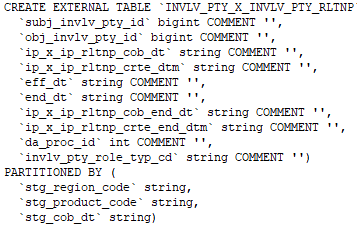
We can create the external table by specifying the EXTERNAL keyword in the Hive create table statement.
Command to create an external table.
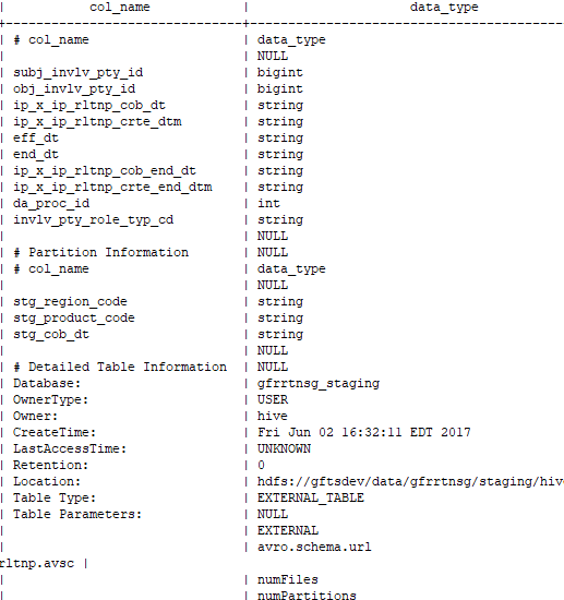
Command to check whether the table created is external or not:-
desc formatted <table_name>
F) Creating a hive environment in scala eclipse:-
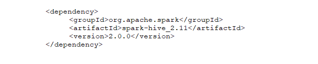
Step 1:- Adding hive maven dependency to the pom file of the eclipse.
Step 2:- Adding spark-session with enableHiveSupport to the session builder.
Step 3:- Command for creating database
Spark.sqlContext.sql(“”” create database gfrrtnsg_staging “””)
This command when executed creates a database in the hive directory of the local system
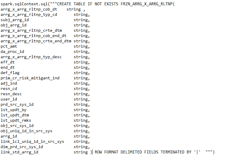
Step 4:- Command for creating a table in eclipse
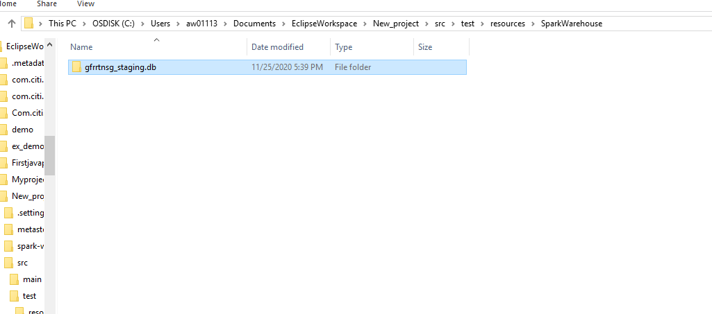
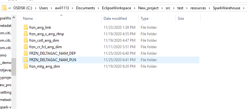
Running this command creates a table in the database folder in the local directory.
After creating a table, you will get a table created inside the database folder in your computer system.
Step 5:- Loading data into tables :-
spark.sqlContext.sql(“”” LOAD DATA INPATH ‘C:sampledata OVERWRITE INTO TABLE frzn_arrg_link “””)
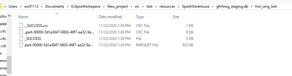
By running this command data gets loaded into tables and thus gives the above output.
Thus, this way data can be stored in hive tables and loaded into data frames and execute your programs.


Very well explained