Pytorch Cheat Sheet for Beginners and Udacity Deep Learning Nanodegree

This cheatsheet should be easier to digest than the official documentation and should be a transitional tool to get students and beginners to get started reading documentations soon.

comments

By Uniqtech

Getting started with Pytorch using a cohesive, top down approach cheatsheet. This cheatsheet should be easier to digest than the official documentation and should be a transitional tool to get students and beginners to get started reading documentations soon. This article is being improved continuously. It is frequently updated and will remain under construction until it is significantly improved. Your feedback is appreciated hi@uniqtech.co and mistakes, typos will be promptly corrected.

Big news: we got published on Medium Machine Learning and Data Science homepage. Please clap ← and comment to show your support. This cheatsheet below is primarily narrative. A PDF JPEG version of a detailed cheatsheet will be released soon, posted in this article. Updated June 18, 2019 to make this cheat sheet / tutorial more cohesive, we will insert code snippets from a medal winning Kaggle kernel to illustrate important Pytorch concepts — Malaria Detection with Pytorch, an image classification, computer vision Kaggle kernel [see Source 3 below] by author devilsknightand vishnu aka qwertypsv.

pytorch cheatsheet for beginners by uniqtech

Pytorch Defined in Its Own Words

Pytorch is “An open source deep learning platform that provides a seamless path from research prototyping to production deployment.”

According to Facebook Research [Source 1], PyTorch is a Python package that provides two high-level features:
Tensor computation (like NumPy) with strong GPU acceleration
Deep neural networks built on a tape-based autograd system
You can reuse your favorite Python packages such as NumPy, SciPy and Cython to extend PyTorch when needed.

Soumith Chintala, Facebook Research Engineer and creator of Pytorch gave some interesting facts about Pytorch: autograd used to be written in python, but the majority (of code) was changed to C++ (for production readiness). He thinks interesting Pytorch 1.0 features are hybrid front end, parsing model for production, using Jit compiler to get models production ready for example. Source: Chintala’s interview with Udacity learning.

Key Features

Component | Description [Source 2]

torch: a Tensor library like NumPy, with strong GPU support
torch.autograd : a tape-based automatic differentiation library that supports all differentiable Tensor operations in torch
torch.jit : a compilation stack (TorchScript) to create serializable and optimizable models from PyTorch code
torch.nn: a neural networks library deeply integrated with autograd designed for maximum flexibility
torch.multiprocessing: Python multiprocessing, but with magical memory sharing of torch Tensors across processes. Useful for data loading and Hogwild training
torch.utils: DataLoader and other utility functions for convenience

Key features: Hybrid Front-End, Distributed Training, Python-First, Tools & Libraries.

These features are elegantly illustrated with side-by-side code example on the features page!

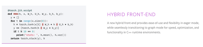
The features page on pytorch documentation shows elegant code sample to illustrated each feature. Also note Python 3 short hand for dot product such as “@”

Hybrid Front-End allows switching between eager mode and (computation) graph mode. Tensorflow used to be graph mode only, which was considered fast and efficient but very hard to modify, prototype and research. This gap is closing since Tensorflow now also offers eager mode (no more session run.)

Distributed Training: supports GPU, CPU and easy switching between the two. (Tensorflow supports TPU in addition. Its own Tensor Processing Unit.)
Python-First: built for python developers. Easily create neural network, run deep learning in Pytorch. Tools & Libraries include robust computer vision libraries (convolutional neural networks and pretrained models), NLP and more.

Pytorch also includes great features like torch.tensor instantiation and computation, model, validation, scoring, Pytorch feature to auto calculate gradient using autograd which also does all the backpropagation for you, transfer learning ready preloaded models and datasets (read our super short effective article on transfer learning), and let’s not forget GPU using CUDA.

When Should You Use Pytorch

AWS google GCP GPU supports Pytorch as first class citizen

Pytorch added production and cloud partner support for 1.0 for AWS, Google Cloud Platform, Microsoft Azure. You can now use Pytorch for any deep learning tasks including computer vision and NLP, even in production.

Because it is so easy to use and pythonic to Senior Data Scientist Stefan Otte said “if you want to have fun, use pytorch”.

Pytorch is also backed by Facebook AI research so if you want to work for Facebook data and ML, you should know Pytorch. If you are great with Python and want to be an open source contributor Pytorch is also the way to go.

Transfer Learning

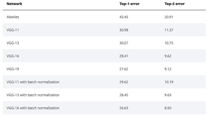
Transfer learning use models to predict the type of the dataset that it wasn’t trained on. It can significantly improve training time and accuracy. It can also help with the situation where available training data is limited. Pytorch has a page dedicated to pre-trained models and its performance across industry standard benchmark datasets. Read more in our transfer learning with Pytorch article.

# pretrained models are at torchvision > models
model = torchvision.models.resnet152(pretrained=False)

Read about all the available models on Pytorch documentation. Note the top-1-error, top-5-error i.e. the performance of the models are also available.

Data Science, Academic Research | Presentation Using Jupyter Notebook

Since Python has a huge developer community, it is easier to find Python talent among students and researchers to transition into Data Science and academic research, even writing production code using Pytorch. Eliminate the need to learn another language. Many data analysts and scientists are already familiar with Jupyter Notebook, on which Pytorch operates perfectly. Read more in our deploying Pytorch model to Amazon Web Service SageMaker.

Pytorch is a Deep Learning Framework

Pytorch is a deep learning framework just like Tensorflow, which means: for traditional machine learning models, use another tool for now. Scikit-learn a Pythonic deep learning framework with extremely easy-to-use API. The documentation is quite good, each page has an example with code snippets at the bottom. Check it out. Did you know many Kaggle users including masters still use sklearn train_test_split() to split and scaler to pre-process data, sklearn Gradient Boosting Tree or Support Vector Machine to benchmark performance, and the top notch high-performance XGBoost is notably missing.

Tensorflow.js and Tensorflow.lite gives Tensorflow wings in the browser and on mobile devices. Apple just announced CreateML for Swift June 2019. Mobile support is not native yet in Pytorch. Do not dispair. Scroll down to read about ONNX an exchange format that is supported by almost of all of the popular frameworks. Pytorch also has a tutorial on moving a model to mobile, though this road is still bit detoured compared to Tensorflow.

Installation Pytorch

For installation tips use the official Pytorch documentation first. https://pytorch.org/get-started/locally/ The above screenshot is an example of available installations.

Using Anaconda to install Pytorch is a great start across all systems including and Windows. We were able to install Pytorch with Anaconda on a gaming computer and start to use its CUDA GPU feature right away. Read our Anaconda Cheatsheet here.

conda install numpy jupyter notebook
conda install pytorch torchvision -c pytorch

Hello World in Pytorch is as easy as launching a Google Colab (yes, right on Google’s turf), and import torch , check out this shared view only notebook. Modern hosted data science notebooks like Kaggle Kernel and Google Colab all come with Pytorch pre-intalled.

Look Ma: deep learning with no server!

Prefer Jupyter Notebook based tutorials instead? Getting started using the Udacity Intro to Pytorch repo, found at the bottom of this article.

Prefer other installation methods? Binaries, from source, and docker image, see Source 2.

Code Snippets from Source 3

import numpy as np
import pandas as pd
import matplotlib.pyplot as plt
import torch
from torch import nn, optim
from torchvision import transforms, datasets, models
from torch.utils.data.sampler import SubsetRandomSampler

import os
print(os.listdir("../input/cell_images/cell_images/"))

import torch is needed for core pytorch tasks. You also see torch neural nets module nn, optimizer optim and computer vision module torchvision, data transformer pipeline transforms , datasets and existing models being imported. In this case the Kaggle team also used a SubsetRandomSampler, you will see in a later snippet how it feeds into the data transformation and loading pipeline.

Data Transformation

Code Snippets from Source 3

Note that the train, test and validation transformers are similar but different. To augment data, training data is randomly rotated, resized and cropped, even vertically flipped (in this case a flipped Malaria cell does not negatively affect classification results). Because test and validation data should mimic real world data, no random noise or flipping is introduced. Just as it is, with center crop. Note that the size must match constantly. Deep Learning is a lot of matrix multiplication. Dimension size always matters. In image classification tasks, we typically want to normalize images according to the pre-trained model or existing dataset we will be using.

# Define your transforms for the training, validation, and testing sets
train_transforms = transforms.Compose([transforms.RandomRotation(30),
 transforms.RandomResizedCrop(224),
 transforms.RandomVerticalFlip(),
 transforms.ToTensor(),
 transforms.Normalize([0.485, 0.456, 0.406], 
 [0.229, 0.224, 0.225])])test_transforms = transforms.Compose([transforms.Resize(256),
 transforms.CenterCrop(224),
 transforms.ToTensor(),
 transforms.Normalize([0.485, 0.456, 0.406], 
 [0.229, 0.224, 0.225])])validation_transforms = transforms.Compose([transforms.Resize(256),
 transforms.CenterCrop(224),
 transforms.ToTensor(),
 transforms.Normalize([0.485, 0.456, 0.406], 
 [0.229, 0.224, 0.225])])

Why the normalization? And what are those strange numbers? Mean and standard deviation.

normalize = transforms.Normalize(mean=[0.485, 0.456, 0.406], std=[0.229, 0.224, 0.225]) # Source 4

Definitely don’t forget ToTensor to transform all to a pytorch tensor.

Why? Because Pytorch expects it. Read this thread by Chimtala smth creator of Pytorch [Source 5].

input image is first loaded to range [0, 1] and then this normalization is applied to RGB image as described here .. torch vision — Datasets, Transforms and Models specific to Computer Vision

All pre-trained models expect input images normalized in the same way, i.e. mini-batches of 3-channel RGB images of shape (3 x H x W), where H and W are expected to be at least 224.

The images have to be loaded in to a range of [0, 1] and then normalized using mean=[0.485, 0.456, 0.406] and std=[0.229, 0.224, 0.225]

An example of such normalization can be found in the imagenet example here [Source 4]

Loading Data Using Train and Test Loaders

train_loader = torch.utils.data.DataLoader(train_data, batch_size=batch_size, num_workers=num_workers)
test_loader = torch.utils.data.DataLoader(test_data, batch_size=batch_size, num_workers=num_workers)

Code Snippet from Source 3

datasets.ImageFolder and the torch.utils.data.DataLoader work together to load train, valid and test data separately, based on batch_size, sampling after data transformation in the previous section. Each dataset has its own loader.

img_dir='../input/cell_images/cell_images/'
train_data = datasets.ImageFolder(img_dir,transform=train_transforms)... # omitted
# convert data to a normalized torch.FloatTensor
... # omitted

# obtain training indices that will be used for validation
... # omitted
print(len(valid_idx), len(test_idx), len(train_idx))

# define samplers for obtaining training and validation batches
train_sampler = SubsetRandomSampler(train_idx)
valid_sampler = SubsetRandomSampler(valid_idx)
test_sampler = SubsetRandomSampler(test_idx)

# prepare data loaders (combine dataset and sampler)
train_loader = torch.utils.data.DataLoader(train_data, batch_size=64,sampler=train_sampler, num_workers=num_workers)
valid_loader = torch.utils.data.DataLoader(train_data, batch_size=32, sampler=valid_sampler, num_workers=num_workers)
test_loader = torch.utils.data.DataLoader(train_data, batch_size=20, sampler=test_sampler, num_workers=num_workers)

Pytorch Model in a Nutshell

Using Sequential is one easy way to quickly define a model. A named ordered dictionary holds all the layers that are encapsulated in nn.Sequential, which is then stored in the model.classifier variable. This is a quick way to define the bare bone of a model but not necessarily the most Pythonic. It helps us illustrate a Python model is consisted of fully connected Linear Layers with shape specified in (row, col) tuples. ReLU activation layers, Dropout with 20% probability and an output Softmax function or LogSoftmax function. Don’t worry about that now. All you need to know is that Softmax is usually the last layer of a Deep Learning model of multi-class classification tasks. The famous ImageNet dataset has 1000+ classes, so the output of Softmax has at least 1000+ components.

A collection of fully connected layers with ReLU activation in between some dropouts and at last, another fully connected linear layer which feeds into a Softmax activation is very typical of a vanilla Deep Learning Neural Network.

from collections import OrderedDictclassifier = nn.Sequential(OrderedDict([
                          ('fc1', nn.Linear(2048, 1024)),
                          ('relu', nn.ReLU()),
                          ('dropout',nn.Dropout(0.2)),
                          ('fc2', nn.Linear(1024, 512)),
                          ('relu', nn.ReLU()),
                          ('dropout',nn.Dropout(0.2)),
                          ('fc3', nn.Linear(512, 256)),
                          ('relu', nn.ReLU()),
                          ('dropout',nn.Dropout(0.2)),
                          ('fc4', nn.Linear(256, 102)),
                          ('output', nn.LogSoftmax(dim=1))
                          ]))model.classifier = classifier

In Pytorch it is easy to view the structure of your model just use print(model_name). More on that later.

Code Snippet in Source 3

As previously mentioned, in transfer learning in the why pytorch section, we can use a pretrained model such as resnet50. Turning gradient off for all layers except the last newly added, fully connected layer.

model = models.resnet50(pretrained=True)

for param in model.parameters():
    param.requires_grad = False # turn all gradient off

model.fc = nn.Linear(2048, 2, bias=True) 
#add new fully connected layer

fc_parameters = model.fc.parameters()

for param in fc_parameters:
    param.requires_grad = True #turning last layer gradient to true
    
model

Note that the last layer is 2048 by 2 because we are classifying just two classes: true or false, malaria or not.

The model variable returns a massive ResNet model structure with our customized last layer.

Downloading: "https://download.pytorch.org/models/resnet50-19c8e357.pth" to /tmp/.torch/models/resnet50-19c8e357.pth
100%|██████████| 102502400/102502400 [00:01<00:00, 89692748.86it/s]

In the code snippet below, we omitted a lot of details to make the model architecture fit on the screen. If you visit the source 3 kernel link, you will see quite a few bottlenecks and sequential layers.

(layer1): Sequential(
    (0): Bottleneck(
      (conv1): Conv2d(64, 64, kernel_size=(1, 1), stride=(1, 1), bias=False)
      (bn1): BatchNorm2d(64, eps=1e-05, momentum=0.1, affine=True, track_running_stats=True)
      (conv2): Conv2d(64, 64, kernel_size=(3, 3), stride=(1, 1), padding=(1, 1), bias=False)
      (bn2): BatchNorm2d(64, eps=1e-05, momentum=0.1, affine=True, track_running_stats=True)
      (conv3): Conv2d(64, 256, kernel_size=(1, 1), stride=(1, 1), bias=False)
      (bn3): BatchNorm2d(256, eps=1e-05, momentum=0.1, affine=True, track_running_stats=True)
      (relu): ReLU(inplace)
      (downsample): Sequential(
        (0): Conv2d(64, 256, kernel_size=(1, 1), stride=(1, 1), bias=False)
        (1): BatchNorm2d(256, eps=1e-05, momentum=0.1, affine=True, track_running_stats=True)
      )
    )

Here we showed that the last customized layer is indeed 2048 by 2. Note that the layer before the average pooling and relu is 2048, hence 2048 by 2.

ResNet(
  (conv1): Conv2d(3, 64, kernel_size=(7, 7), stride=(2, 2), padding=(3, 3), bias=False)
... #omitted
    ... #omitted
      (bn3): BatchNorm2d(2048, eps=1e-05, momentum=0.1, affine=True, track_running_stats=True)
      (relu): ReLU(inplace)
    )
  )
  (avgpool): AvgPool2d(kernel_size=7, stride=1, padding=0)
  (fc): Linear(in_features=2048, out_features=2, bias=True)
)

Pytorch Training Loop

The training loop is perhaps the most characteristic of Pytorch as a deep learning framework. In Sklearn can make it go away with fit and in Tensorflow with transform. In Pytorch this part is much more involved.

model.train() tells your model that you are training the model. So effectively layers like dropout, batchnorm etc. which behave different on the train and test procedures know what is going on and hence can behave accordingly.

More details: It sets the mode to train (see source code). You can call either model.eval() or model.train(mode=False) to tell that you are testing. It is somewhat intuitive to expect trainfunction to train model but it does not do that. It just sets the mode.

model.eval() will notify all your layers that you are in eval mode, that way, batchnorm or dropout layers will work in eval model instead of training mode.

torch.no_grad() impacts the autograd engine and deactivate it. It will reduce memory usage and speed up computations but you won’t be able to backprop (which you don’t want in an eval script). — albanD

Code Snippet Training Loop Source 3

use_cuda = torch.cuda.is_available()
if use_cuda:
    model = model.cuda()
criterion = nn.CrossEntropyLoss()
optimizer = optim.SGD(model.fc.parameters(), lr=0.001 , momentum=0.9)

Check CUDA availability, set criterion to CrossEntropyLoss(), and optimizer to Stochastic Gradient Descent for example before starting to train. Note that the learning rate starts very small at about lr=0.001.

Note that the training loop typically takes in number of epochs, model architecture optimizer and criterion. The loss has to be zero’ed out first at the start of every loop! The big loop iterates through the number of epochs. In each epoch, we put the model into training model model.train(), move model and data to CUDA if needed, optimizer.zero_grad() zero out the gradient before starting, predict output, use criterion to calculate loss, loss.backward to calculate the delta weight change based on optimizer, optimizer.step() to take one backward step to update weight. When validating, turns the model to eval model model.eval(). Save the model if validation loss has decreased, keep track of the lowest validation loss.

def train(n_epochs, model, optimizer, criterion, use_cuda, save_path):
    """returns trained model"""
    # initialize tracker for minimum validation loss
    valid_loss_min = np.Inf
    
    for epoch in range(1, n_epochs+1):
        # initialize variables to monitor training and validation loss
        train_loss = 0.0
        valid_loss = 0.0
        
        ###################
        # train the model #
        ###################
        model.train()
        for batch_idx, (data, target) in enumerate(train_loader):
            # move to GPU
            if use_cuda:
                data, target = data.cuda(), target.cuda()

            # initialize weights to zero
            optimizer.zero_grad()
            
            output = model(data)
            
            # calculate loss
            loss = criterion(output, target)
            
            # back prop
            loss.backward()
            
            # grad
            optimizer.step()
            
            train_loss = train_loss + ((1 / (batch_idx + 1)) * (loss.data - train_loss))
            
            if batch_idx % 100 == 0:
                print('Epoch %d, Batch %d loss: %.6f' %
                  (epoch, batch_idx + 1, train_loss))
        
        ######################    
        # validate the model #
        ######################
        model.eval()
        for batch_idx, (data, target) in enumerate(valid_loader):
            # move to GPU
            if use_cuda:
                data, target = data.cuda(), target.cuda()
            ## update the average validation loss
            output = model(data)
            loss = criterion(output, target)
            valid_loss = valid_loss + ((1 / (batch_idx + 1)) * (loss.data - valid_loss))

            
        # print training/validation statistics 
        print('Epoch: {} \tTraining Loss: {:.6f} \tValidation Loss: {:.6f}'.format(
            epoch, 
            train_loss,
            valid_loss
            ))
        
        ## TODO: save the model if validation loss has decreased
        if valid_loss < valid_loss_min:
            torch.save(model.state_dict(), save_path)
            print('Validation loss decreased ({:.6f} --> {:.6f}).  Saving model ...'.format(
            valid_loss_min,
            valid_loss))
            valid_loss_min = valid_loss
            
    # return trained model
    return model

Developer Tools

Train on more than one GPU

Training Loops:

Train and Forward

Free GPU in the Cloud

Thanks you new cloud technology like Google Colab. Once you set up the notebook, you can continue train and monitor on your mobile devices! Cloud choices including Google Colab, Kaggle, AWS. Local choices including your own laptop and your gaming computer.

We repurposed an msi NVIDIA GTX 1060 previously for Assassin’s Creed Origin :D If you want to know more let us know.

Be able to train on a GPU locally has been a major advantage. We were able to iterate through parameter tuning combinations fast without interuption. Google Colab has a 12-hour timeout as well as a 12GB quota limit. If you are an advanced user, be sure to avoid constantly downloading the dataset, instead store it in your Google Drive. After deleting your model in Google Drive, be sure to empty trash to actually delete it.

Regardless of where the model is trained, if the training loss has gone down a lot near zero, but the validation loss does not decrease (there’s no test dataset), you may want to watch out your model is overfitting and it may be memorizing training data. Halt and tune your parameters. Even if you achieve 99% accuracy your model may not generalize, hence it’s a possibility that it cannot be used else where. This paragraph of information is especially relevant for Udacity students doing scholarship challenges and nanodegrees. Be very suspicious of 99% accuracy, but do a brief dance to celebrate first.

Forwarding

Pytorch forward pass will actually calculate y = wx + b before that we are just writing placeholders.

Useful Pytorch Libraries and Modules and Installations.

import torch
import torchvision
from torchvision import datasets, transforms, models
import torch.nn.functional as F
from collections import OrderedDict
from torch import nn
from torch import optim

The Torchvision module is quite powerful. It has image processing and data processing codes, Convolutional Neural Nets (CNN), and other pretrained models like ResNet and VGG.

Transformation

transforms.ToTensor() convert data array to Pytorch tensor. Advantage include easy to use in CUDA, GPU training.
Developers can build transformation and transformation pipelines in Pytorch. Pipeline is a fancy way to say transformations that are chained together, and performed sequentially.

Pytorch Convolutional Neural Networks (CNN)

This section is under construction… check back soon.

Use Convolutional Neural Networks to complete computer vision, image recognition tasks. The transformation and data augmentation APIs are very important, especially when training data is limited. Alternatively one can also use many of the preloaded model architectures — read our transfer learning section.

import torch
import numpy as np
from torchvision import datasets
import torchvision.transforms as transforms

Maxpooling layer discards detailed spatial information contained in the original image.

Inspect Pytorch Models

First init the model.

vgg16 = models.vgg16(pretrained=True)
print(vgg16)

In Pytorch, use print(model_name) to print out the model and architecture of the model. You can easily see what the model is all about.

VGG(
  (features): Sequential(
    (0): Conv2d(3, 64, kernel_size=(3, 3), stride=(1, 1), padding=(1, 1))
    (1): ReLU(inplace)
    (2): Conv2d(64, 64, kernel_size=(3, 3), stride=(1, 1), padding=(1, 1))
...
    (24): Conv2d(512, 512, kernel_size=(3, 3), stride=(1, 1), padding=(1, 1))
...
    (29): ReLU(inplace)
    (30): MaxPool2d(kernel_size=2, stride=2, padding=0, dilation=1, ceil_mode=False)
  )
  (classifier): Sequential(
    (0): Linear(in_features=25088, out_features=4096, bias=True)
    (1): ReLU(inplace)
    (2): Dropout(p=0.5)
    (3): Linear(in_features=4096, out_features=4096, bias=True)
    (4): ReLU(inplace)
    (5): Dropout(p=0.5)
    (6): Linear(in_features=4096, out_features=1000, bias=True)
  )
)

Note that each layer is named (numbered and can be queried by this index).We used ellipsis to omit model details so that the VGG model can fit on the screen.

Pro tip: inspecting the model architecture is a must. Transfer learning, in a nutshell, is about modifying the last few classifier layers. Read more in our transfer learning article.

Pro tip: for Tensorflow use keras model.summary() to review the entire model architecture. It even outputs number of parameters and dimensions.

Advanced Features

Pytorch Versions

For Udacity projects, not all nanodegrees have moved to Pytorch 1.0 It is important to use the right version for the right project. You may also need to change the Kernel in Jupyter Notebook to use corresponding version of Python. Udacity projects have moved onto Python3. Not all projects in the real world has migrated to Python 3. But it’s about time to move on from Python 2.

Using CUDA

Though we decided to put CUDA in the advanced section, but the reality is CUDA is so easy to use. Just use it… today! With Anaconda, Pytorch, and CUDA, we were able to turn a gaming computer with an NVDIA graphics card into a home deep learning powerhouse. No configuration needed! It just works. The framework just works on a windows machine! (It is an msi NVIDIA GTX 1060 previously for Assassin’s Creed Origin :D If you want to know more let us know.)

gpu_is_avail = torch.cuda.is_available()if not gpu_is_avail:
     print('CUDA is NOT available.')
else:
     print('CUDA is available. ')device = torch.device(“cuda” if torch.cuda.is_available() else “cpu”)

One common error of using CUDA with Pytorch is not moving both the model and the data to CUDA. And when needed move both of them back to CPU. Generally your model and data should always live in the same space.

Deploying Pytorch in Production: There are two methods of turning existing Pytorch models to production ready deployment trace and scripting. Tracing does not support complex models with control flow in the code. Scripting supports Pytorch codes with control flow but supports only a limited number of Python modules.

Choosing the best Softmax result: in multi-class classification, the activation Softmax function is often used. Pytorch has a dedicated function to extract top results — the most likely class from Softmax output. torch.topk(input, k, dim) returns the top probability.

torch.topk(input, k, dim=None, largest=True, sorted=True, out=None) -> (Tensor, LongTensor)
Returns the k largest elements of the given input tensor along a given dimension.
If dim is not given, the last dimension of the input is chosen.
If largest is False then the k smallest elements are returned.

Consume Pytorch Models on Other Platforms

import torch.onnx
  import torchvision

  dummy_input = torch.randn(1, 3, 224, 224)
  model = torchvision.models.alexnet(pretrained=True)
  torch.onnx.export(model, dummy_input, "alexnet.onnx")

“Export models in the standard ONNX (Open Neural Network Exchange) format for direct access to ONNX-compatible platforms, runtimes, visualizers, and more.” — Pytorch 1.0 Documentation

More on Pytorch Transfer Learning

To use an existing model is equivalent to freeze some of its layers and parameters and not train those. Turn off training autograd by setting require_grad to False.

for param in model.parameters():
 param.requires_grad = False

Hyperparameter Tuning

In addition to using the right optimizer and adjusting learning rate according. You can use the learning rate scheduler to dynamically adjust your learning rate.

#define scheduler
scheduler = lr_scheduler.StepLR(optimizer, step_size=3, gamma=0.1)

Read more about scheduler here.

Model and Check Point Saving

Save and Load Model Checkpoint

Pro tip: Did you know you can save and load models locally and in google drive? This way you don’t have to start from scratch every time. For example, if you already trained 5 epochs. You can save the weights and train another 5 epochs. Now you did 10 epochs total! Very convenient. The free GPU resources time out and get erased very often. Remember incremental training is possible.

You can also save a checkpoint and load it locally. You may see both extension .pt and .pth .

# write and then use your custom load_checkpoint function
model = load_checkpoint('checkpoint_resnet50.pth')
print(model)# use pytorch torch.load and load_state_dict(state_dict)
checkpt = torch.load(‘checkpoint_resnet50.pth’)
model.load_state_dict(checkpt)#save locally, map the new class_to_idx, move to cpu
#note down model architecturecheckpoint['class_to_idx']
model.class_to_idx = image_datasets['train'].class_to_idx
model.cpu()
torch.save({'arch': 'resnet18',
           'state_dict': model.state_dict(),
           'class_to_idx': model.class_to_idx},
           'classifier.pth')

Code Snippet from Source 3

model.load_state_dict(torch.load('malaria_detection.pt'))

Note you must save any checkpoint on Google Colab to your Google Drive, else your data may be erased every 12 hours or sooner. Though the GPU access is free, the storage is temporary on Google Colab.

Making Predictions with Pytorch

Here’s what we don’t like about Pytorch. Making predictions with Pytorch seems to be a bit patched together. Writing your own training loop seems easy-to-customize, though it is harder to write than Tensorflow, it makes sense to trade a bit of discomfort for customization. But prediction is strange which some functions that appear to be hacked together. See these code snippets below to see what we mean:

Code Snippets from Source 3:

def test(model, criterion, use_cuda):

   ... #omitted
        # convert output probabilities to predicted class
        pred = output.data.max(1, keepdim=True)[1]
        # compare predictions to true label
        correct += np.sum(np.squeeze(pred.eq(target.data.view_as(pred))).cpu().numpy())
        total += data.size(0)
    .... #omitteddef load_input_image(img_path):    
    image = Image.open(img_path)
    prediction_transform = transforms.Compose([transforms.Resize(size=(224, 224)),
                                     transforms.ToTensor(), 
                                     transforms.Normalize([0.485, 0.456, 0.406], 
                                                          [0.229, 0.224, 0.225])])

    # discard the transparent, alpha channel (that's the :3) and add the batch dimension
    image = prediction_transform(image)[:3,:,:].unsqueeze(0)
    return imagedef predict_malaria(model, class_names, img_path):
    # load the image and return the predicted breed
    img = load_input_image(img_path)
    model = model.cpu()
    model.eval()
    idx = torch.argmax(model(img))
    return class_names[idx]

output.data.max, np.sum(np.squeeze()) , cpu().numpy(), .unsqueeze(0), torch.argmax …WTF?! It’s super frustrating.

The important take away is: we are working with logits converted to probabilities here, and there are tensors that need to be turned into matrices and extra brackets removed. We need to know which one is most likely class using max or argmax. We need to move tensors back to CPU so cpu() and tensor needs to be turned into ndarray for ease of computation so numpy().

Pytorch is a deep learning framework, and deep learning is frequently about matrix math, which is about getting the dimensions right, so squeeze and unsqueeze have to be used to make dimensions match.

>>> import torch
>>> import numpy as np
>>> test = torch.tensor([[1,2,3]])
>>> np.squeeze(test)
tensor([1, 2, 3])
>>> torch.tensor([1]).unsqueeze(0)
tensor([[1]])

This part of the cheatsheet will save you a lot of headache and you are welcome! np.squeeze() removed the extra set of [] and an extra dimension out of [[1,2,3]] of shape (1, 3). Now it is just (3,). A

And unsqueeze made [1] shape of (1,) to [[1]] shape (1,1).