


If data acquisition is the very first step of any machine learning project, unfortunately, data doesn’t always come with the label of interest for the task at hand. It is often a very cumbersome task to (correctly!) label the data — and that’s where active learning comes in.
Instead of randomly labeling samples, active learning strategies strive at selecting the next most useful sample to label. There are many such strategies depending on various notions of usefulness; for example, uncertainty aims at selecting samples that are difficult for the model to classify, while density-based ones aim at exploring the space of features. For a general introduction to active learning, we highly recommend this blog post series.
A good way to step into the domain is to take a look at the available implementations. This blog post will present a high-level (non-exhaustive) perspective on existing active learning packages and how they compare, diving into some specific features of those packages. We will cover the simplest approaches available in each Python active learning package, review some aspects of the code, and quickly present the most cutting-edge methods proposed.

The Contenders
modAL is the lightest package, and it features the most common query sampling techniques through Python functions along with a wrapper object that exposes them as a scikit-learn estimator. modAL has a strong focus on approaches mixing several classifiers (query by committee).
Libact’s main advantage is to feature an “active learning by learning” strategy. It consists of using a multi-armed bandit strategy over existing query sampling strategies to dynamically select the best approach. Libact has a strong focus on performance and therefore uses C code, which can be tricky to install.
Alipy is probably the package that features the highest number of query strategies, most of them being methods in the laboratory of the main contributors.
Testing Protocol
The tests presented in this blog post were done on two datasets:
- A synthetic dataset generated using sklearn.datasets.make_classification
- 10 classes
- 1,000 samples
- 20 active learning iterations
- 20 samples per batch
2. The MNIST dataset available through sklearn.datasets.load_digits
- 10 classes
- 1,797 samples
- 16 active learning iterations
- 50 samples per batch
Datasets were split into a train and a test dataset, both containing 50% of the samples. The scores reported below are accuracy scores measured on the test set exclusively. Experiments use the following protocol:
- Each experiment is run 20 times while changing the seed.
- The seed is used to generate the data in the synthetic dataset, and to select the first batch of samples in the MNIST experiment.
- Each curve represents the average of the results over the 20 runs. Confidence intervals are 10% and 90% quantiles.
- The model used is a scikit-learn SVC with default parameters: RBF kernel, C=1.0. In order to ensure that our results are not classifier-dependent, results were repeated using other parameters, and other classifiers and did not differ significantly.
Uncertainty-Based Methods
Model uncertainty is the most natural active learning strategy. It is based on the intuition that the samples that can bring the most information to the model are the ones on which it has the least confidence. These samples are identified by looking at the classification probabilities.
Since these strategies are common and all packages use the same definitions, we did not investigate it — we simply used it to sanity check our pipelines and protocol.
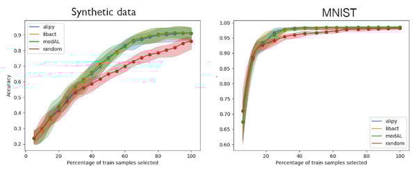
Figure 1. Active learning using smallest margin query sampling on synthetic data and MNIST
In both tasks (Figures 1), the active learning strategy outperforms random. The difference is more striking on synthetic data, which is probably because the problem is harder (twice the number of classes with twice the number of samples).
Taking Data Distribution Into Account Through Density
Active learning aims at making the best use of labeled data. However, unlabeled data also holds information (such as the distribution of the samples), and this information is typically used in unsupervised and semi-supervised methods.
An assumption commonly made in unsupervised learning is that the likelihood for two samples to belong to the same class is proportional to their similarity according to a given distance measure. If this holds, it means that a cluster of samples is likely to have the same label and can be represented by one of the samples.
Active learning strives to select a subset of the training set that best represents the whole dataset. Following this logic, we can hypothesize that selecting samples located in areas with a high density of points better represent the dataset.
There is no general mathematical definition of density, so each package has chosen its own way to compute density:
- ModAL defines the density of a sample as the sum of its distance to all the other samples, although we chose for our test to follow [2], referred in modAL, that defines it as the sum of the distance to unlabeled samples. A lower distance means a higher density. We used the cosine and euclidean distances in our examples.
- Alipy defines the density as the average distance to the 10 nearest neighbors based on [1]. We expect this approach to be more robust than modAL’s, but the choice of 10 neighbors seems arbitrary and is not exposed to the user.
- Libact proposes a first approach based on K-Means using cosine similarity, close to modAL’s one. Libact’s documentation references the method as coming from [2], but the formula is slightly different than the one in the paper (they don’t provide an explanation as to why).
- Libact features a second method based on [6]. This method performs a clustering of the data and fits a GMM on the clusters to estimate the global density through the mixing probability and a score for each point in the cluster using the pdf (refer to the original paper for a complete description). Note that the original approach uses K-medoids, but that for now, Libact uses a K-Means.
A quick glance reveals that modAL opted for the most natural and simple definition, even though it does not scale. Libact and alipy opted for more sophisticated clustering-based approaches that are more likely to scale, but the hard-coded parameters raise the question of generalization.
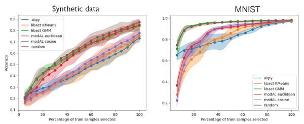
Figure 2. Active learning using density-based query sampling on synthetic data and MNIST
The first point to notice in both experiments is that random is at least as good as all density-based strategies, which makes us question whether density is a good strategy at all! In fact, targeting zones of high density may force the system to explore all data clusters, but it also constrains the selection of samples in the center of these clusters where the decision boundaries rarely lie, contradicting the uncertainty-based approach.
On this task, Libact’s GMM performances are on par with random. It could be that this method is more robust than the others and able to perform better on this task, or just that it has a behavior equivalent to random (in which case it may not be useful). More experiments on other tasks would be required to come to a definitive conclusion.
ModAL’s euclidean-based approach seems like a good tradeoff in both experiments. The cosine based one (along with alipy’s) is less convincing on the synthetic data set, but this may be due to the way the synthetic data is generated. Other approaches have poorer performance, and in the end, alipy’s and KMeans-based libact’s approaches are bad on both tasks — but we cannot exclude that they could do better if the hard-coded clustering hyperparameters were tuned.
It is also worth noticing that modAL’s method has suspiciously low performance when less than 20% of the dataset is labeled. The reason may be that libact’s and alipy’s approach are clustering-based and thus promote an exploration of the sample space, while modAL’s method is stuck in high-density areas.
Batch Sampling Methods
With the rise of deep learning, training models became more and more expensive, both in terms of time and computation resources. A focus has thus been put in developing batch active learning methods instead of the previous online methods.
Indeed, selecting samples independently can be suboptimal compared to random sampling. Imagine that one is trying to classify fruits and has already randomly labeled some samples. Our model may struggle to differentiate between apricots and peaches, coconut and passionfruit, etc. In that case, an uncertainty-based query sampler will select a set of samples from the hardest problem (e.g., apricot vs. peaches).
We expect that a batch method in the same situation would select some samples from each of these grey areas. Batch methods usually mix uncertainty scores with spatial approaches, such as the density ones presented before:
- modAL proposes the ranked batch-mode active learning method that selects samples using uncertainty score but also strives to maximize the distance to already-labeled points. It is called ranked because this method is based on an iterative process where the previously selected item is taken into account: the algorithm starts by selecting a sample on which the model is uncertain and that is far away from already-labeled samples. Then, it considers this selected sample as labeled to select the next one. The process is repeated until batch size is reached. In the end, a partial order is established between samples.
- For libact, we use the two same methods described in the density section defined here and here. In fact, they allow us to mix density and uncertainty approaches by making a weighted sum of both scores. It is not a proper batch sampling method, but this is what is closest among the methods proposed by this package.
- Alipy proposes a batch method that has not been considered for this study since it only works for binary classification problems.
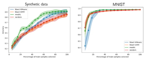
Figure 3: Active learning using batch query sampling on synthetic data and MNIST
ModAL is the winner in both experiments, although the trend is less obvious on MNIST. As for libact’s GMM, we observe a performance similar to random, as in figure 2. On MNIST, we note that libact’s KMeans is now performing badly with less annotated data. It reveals how dataset-dependent active learning may be and how difficult is it to chose the best query sampling method.
Meta Active Learning
There are other more advanced query sampling approaches available in these packages. In particular, the ones where a model is used to learn how to do the query sampling. These methods have different approaches, so comparing is not pertinent. Also, benchmarking them is out of the scope of a single blog post. So if you want to know more, please refer to their associated papers.
Learning Active Learning [4] (libact)
Learning active learning is a strategy made to get the best out of several query sampling strategies. Behind the scenes, it uses a multi-arm bandit approach to determine which is the best method depending on the situation. The bandit uses the Importance Weighted Accuracy as a reward, an unbiased estimator of the test accuracy. This is interesting, as most of the approaches use error reduction as a reference score to estimate the performance of a query method.
The main cost of this strategy is scoring the whole dataset at each iteration. In most of the reported experiments, this method manages to make use of the most efficient query sampling on which it is based. One drawback — obviously — is that it is rarely better than the samplers it is based on.
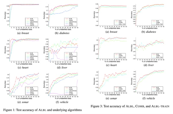
Figure 4. Original results as reported in [4]. Figure numbers are the ones from the original paper.
Active Learning From Data [5] (alipy)
The idea behind active learning from data is to be able, given the current state of an active learning experiment, to predict the error reduction brought by each unlabeled sample. In this method, the “current state” of the experiment is represented by the model learned on the already labeled data. So in order to estimate the impact of one sample on this model, the authors propose to look at some stats of the learning set, the inner state of the model, and the predictions made by that model for the given sample.
More precisely, the proposed implementation uses a random forest as classifier and predicts error reduction based on:
- Feature extracted on the training set:
- The proportion of positive labels (i.e., > 0). This is the only indicator we have trouble understanding, since 0 does not seem to be a special class label.
- The number of already-labeled data points.
2. Features extracted from the model:
- Out-of-bag score estimate.
- Standard deviation of feature importance.
- The average depth of the trees in the forest.
3. The predictions of each tree for the current sample:
- The average probability for each class.
- The standard deviation for each class across all trees.
- The average of the standard deviation of all classes for all samples.
The model can be trained on already-labeled data, but alipy also ships pre-trained models that, according to them, can perform well on a variety of tasks. Similar to the method provided in libact, the results are significantly better than other methods on only a very limited subset of problems.
 Figure 5: Results of the original paper [5] on synthetic data
Inter-Operability With Scikit-Learn
In the past years, Scikit-learn managed to become a machine learning reference both in academia and industry. One of the reasons for this success is probably due to its careful minimalistic design [3] that covers a wide range of use cases while allowing great flexibility.
Scikit-learn relies on a base estimator interface that exposes three methods:
- __init__ The parameters of a model are specified through the constructor. No data-specific information is passed during this phase.
- fit The fit method must be given all the necessary information for the model to be learned. It includes the training data, of course, the labels for a supervised model, and any other data-specific parameter.
- predict The predict method performs the inference. It returns label prediction. Any additional insight that may be useful to the user is stored in the object in a property ending with an underscore.
Scikit-learn is designed for maximum code reusability. For instance, in model family — supervised, semi-supervised, clustering, etc .— all methods share the same interface. This makes it easier to change models and compare them.
With its minimalistic interface, modAL is the closest to what we would expect from a scikit-learn compatible active learning package. Strategies are represented by functions, which is accepted. What is lacking though (in my opinion) is a flag allowing one to get more information about the results. For example, one may want to use the uncertainty scores for something other than selecting queries — sample weighting, for example. This is, unfortunately, not possible.
Alipy objects follow the philosophy of minimalistic common interface. However, some of them require the data to be passed in the constructors, which is not forbidden in the scikit-learn paradigm. Finally, libact does not follow the scikit-learn interface, but it has a very close one. It ships its own models and offers a wrapper to use scikit-learn ones. What is surprising, though, is that libact sometimes performs computation in the constructor of some methods. For example, Density Weighted Uncertainty Sampling performs a KMeans directly into the constructor. An odd thing is that the same class compute scores but does not support the “return_scores” flag to be able to recover them.
Experimental Frameworks
Questions that are paramount when doing active learning are:
- When should one start doing active learning as opposed to random labeling ?
- When should one stop?
- How does one know that active learning is doing better than random?
So far, we have focused on query sampling methods. We are now taking a look at the active learning experimental machinery provided by each library.
Libact does not — per se — provide an experimental framework. The active learning loop is left to the user. There are only two simple helpers called labelers: an ideal labeler that simulates perfect annotation, and a manual one that displays features in a matplotlib figure and asks for the label using input (so mainly targeted at images).
ModAL does not provide an experimenter either, but a global object (ActiveLearner) allows for easy experimentation with the query sampling techniques proposed. Since properly handling the indexing is maybe one of the main source of errors in active learning, it is useful to be able to rely on a tested package for that.
Alipy offers a full experimental framework. It provides an AlExperiment object, allowing the running of a full experiment but also the building blocks to build its own:
- Utils to split datasets
- Various types of oracles to test the robustness of query sampling methods
- A caching system to store intermediate results during an experiment
- A set of simple stopping criteria — fix cost, fix samples to label, etc.
- An experiment analyzer that provides insights and plots from an experiment
Takeaways
Through our experiments, we have built some takeaways on active learning experiments:
- It is still unclear when a given active learning strategies prevail, and it is often hard to find strategies consistently better than the very naive ones, such as uncertainty-based. And even when they do, the difference is not always worth the effort of deploying them.
- Active learning seems to be more useful when the number of classes is high. We have observed no significant improvement on binary classification problems.
- When there is no available labeled data to start with, we unsurprisingly found that a random strategy performs the best.
- No framework has addressed the problematic of choice-of-query sampling method, depending on the problem (which is complicated for beginners in the domain).
Given our experiments with the three main Python active learning packages, here are our recommendations:
- ModAL provides straightforward methods in a lightweight and simple interface. If one’s goals is to quickly experiment with active learning, we would recommend this package. It is also the only one to feature bayesian methods.
- Alipy features more advanced techniques, but in most of our benchmarks, they were the slowest to run. We would recommend alipy if looking for one of the exclusive methods it features — such as self-paced active learning — or for people who are looking for a fully featured active learning framework. In fact, their AlExperiment object allows the setting up of experiments in minutes
- Finally, libact focuses on performance and provides high-performance implementations of active learning methods. We are still not convinced by the usefulness of the most complex approaches, such as the GMM based one.
Our series of blog posts about active learning will continue, so be on the lookout for our next article on the lessons we learned from reproducing a strategy mixing uncertainty and diversity techniques.