Applying Data Science to Cybersecurity Network Attacks & Events
Check out this detailed tutorial on applying data science to the cybersecurity domain, written by an individual with backgrounds in both fields.
By Aakash Sharma, Data Scientist
The cyber world is such a vast concept to comprehend. At the time, I decided I wanted to get into cybersecurity during my undergrad in college. What intrigued me was understanding the concepts of malware, network security, penetration testing & the encryption aspect that really plays a role in what cybersecurity really is.
Being able to protect the infrastructure is important but interesting nonetheless. Sure there is coding but I never really learned how we can implement code into cybersecurity principles. This is what I really want to know next that could stretch my knowledge in information technology & computer science. I learned more about coding especially in Python. I dabbled a little in Scala & I already had a good foundation of Sequel & Java applications during my undergrad that learning it during my boot camp allowed me to feel a little more comfortable with it.
The data science immersive program taught me how to gather data through Sequel, JSON, HTML or web-scrapping applications where I went into cleaning the data & then applying Python related code for statistical analysis. I then as able to model the data to either find trends, make predictions, or provide suggestions/recommendations. I wanted to apply this to my background in Cisco NetaCad, cybersecurity principles & software development

I then wanted to relate this to my cybersecurity background. I decided to gather data from Data.org regarding a ton of cyber attacks regarding the Federal Communications Commission (FCC). In this blog post, I decided to write about how I was able to connect my data science knowledge to my cybersecurity background in real world industries. I will provide some background of the project, a code along & some insight into what the FCC could do to better understand the data as I did. This could be useful for future situations or other government related cybersecurity projects.
So the FCC, to the best of my knowledge, follows the CSRIC Best Practices Search Tool which allows you to search CSRIC’s collection of Best Practices using a variety of criteria including Network Type, Industry Role, Keywords, Priority Levels & BP Number.
The Communications Security, Reliability & Interoperability Council’s (CSRIC) mission is to provide recommendations to the FCC to ensure, among other things, optimal security & reliability of communications systems, including telecommunications, media & public safety.
CSRIC’s members focus on a range of public safety & homeland security-related communications matters, including: (1) the reliability & security of communications systems & infrastructure, particularly mobile systems; (2) 911, Enhanced 911 (E911), & Next Generation 911 (NG911); & (3) emergency alerting.
The CSRIC’s recommendations will address the prevention & remediation of detrimental cyber events, the development of best practices to improve overall communications reliability, the availability & performance of communications services & emergency alerting during natural disasters, terrorist attacks, cyber security attacks or other events that result in exceptional strain on the communications infrastructure, the rapid restoration of communications services in the event of widespread or major disruptions & the steps communications providers can take to help secure end-users & servers.
The first step for me in tackling this project was understanding what I needed to accomplish & what kind of direction this project had me taking. I had remembered that I needed to provide recommendations to the FCC to ensure optimal security & reliability of communication systems in telecommunications, media & public safety.
There are different approaches I had taken into account when attempting this project. The 1st is diving straight in in order to better understand the data itself where I focused on just the priority of the event & applying a ton of machine learning classification models to it. The 2nd approach was being able to apply natural language processing techniques on the description of the event & see how that correlates to the priority of the event.
With this we can make predictions & following that, recommendations to better prevent, understand or control the event. My idea is if we can focus on the more critical events by fixing the less complex ones, we can save enough assets to further improve the systems to combat the more complex ones.
What is needed:
- A Python IDE
- Machine Learning & Statistical Packages
- Strong knowledge in Data Science Concepts
- Some knowledge in cybersecurity & network related concepts
Let’s begin! Let’s first start by importing any packages we intend on using, I usually copy & paste a list of useful modules that has helped me with previous data science projects.
import pandas as pd
import numpy as np
import scipy as sp
import seaborn as sns
sns.set_style('darkgrid')
import pickle
import regex as re
import gensimfrom nltk.stem import WordNetLemmatizer
from nltk.tokenize import RegexpTokenizer
from nltk.stem.porter import PorterStemmer
from nltk.stem.snowball import SnowballStemmer
from nltk.corpus import stopwords
from sklearn.feature_extraction import stop_words
from sklearn.feature_extraction.text import CountVectorizer, TfidfVectorizerimport matplotlib.pyplot as plt
from sklearn.model_selection import train_test_split, GridSearchCV
from sklearn.preprocessing import StandardScaler
from sklearn.naive_bayes import MultinomialNB
from sklearn.linear_model import LinearRegression,LogisticRegression
from sklearn import metrics
from sklearn.ensemble import RandomForestClassifier, BaggingClassifier, AdaBoostClassifier, GradientBoostingClassifier
from sklearn.neighbors import KNeighborsClassifier
from sklearn.tree import DecisionTreeClassifier
from sklearn.pipeline import Pipeline
from keras import regularizers
from keras.models import Sequential
from keras.layers import Dense, Dropoutimport warnings
warnings.filterwarnings('ignore')%matplotlib inline
We then need to load in the data & view it by:
# Loads in the data into a Pandas data frame
fcc_csv = pd.read_csv('./data/CSRIC_Best_Practices.csv')
fcc_csv.head()
Now that we have our data we can explore, clean & understand the data. Below, I have provided a function for basic data exploratory analysis. We want to do this to fully understand the data we’re dealing with & what the overall goal needs to be met.
The following function will allow us to view any null values, replace any blank spaces with an underscore, reformat the data frame index, see the data types for each column, display any duplicated data, describes the statistical analysis of the data & checks the shape.
# Here is a function for basic exploratory data analysis:def eda(dataframe):
    # Replace any blank spaces w/ a underscore.
    dataframe.columns = dataframe.columns.str.replace(" ", "_")
    # Checks for the null values.
    print("missing values{}".format(dataframe.isnull().sum().sum()))
    # Checks the data frame range size.
    print("dataframe index: {}".format(dataframe.index))
    # Checks for data types of the columns within the data frame.
    print("dataframe types: {}".format(dataframe.dtypes))
    # Checks the shape of the data frame.
    print("dataframe shape: {}".format(dataframe.shape))
    # Gives us any statistical information of the data frame.
    print("dataframe describe: {}".format(dataframe.describe()))
    # Gives us the duplicated data of the data frame. print("duplicates{}".format(dataframe[dataframe.duplicated()].sum()))
    # A for loop that does this for every single column & their
    # values within our data frame giving us all unique values.
    for item in dataframe:
        print(item)
        print(dataframe[item].nunique())# Let's apply this function to our entire data frame.
eda(fcc_csv)
Based off of the data we say that this was a unbalanced classification problem! What we need to do next is eliminate any “NaN” or null values & somewhat balance our class. Based off of our exploratory data analysis, we can see that most of the data has “NaN” values in the object type columns. We can fix this with the following function below!
# Here's a function to convert NaN's in the data set to 'None' for
# string objects.
# Just pass in the entire data frame.
def convert_str_nan(data):
    return data.astype(object).replace(np.nan, 'None', inplace = True)convert_str_nan(fcc_csv)
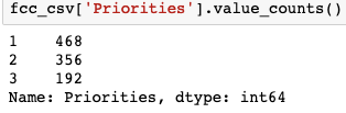
Looking at the priority column(s), we have a object related column that ranks the severity of the event to important, highly important & critical. Another column that corresponds to that priority column ranks them 1–3, with 1 being important, 2 as highly important & 3 being critical. Based off of the variety of priorities, we see that the data is unbalanced. We fix this by renaming our column for better understand & then balancing it where we focus on the highly important & critical events.
# Let's rename the 'Priority_(1,2,3)' column so we can utilize it.
fcc_csv.rename(columns = {
'Priority_(1,2,3)': 'Priorities'
},
inplace = True)# Let's view the values & how the correspond to the 'Priority'
# column.
fcc_csv['Priorities'].value_counts()# We notice that we have an unbalanced classification problem.
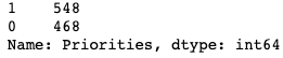
# Let's group the "Highly Important" (2) & "Critical" (3) aspects
# because that's where we can make recommendations.
# Let's double check that it worked.
fcc_csv['Priorities'] = [0 if i == 1 else 1 for i in fcc_csv['Priorities']]
fcc_csv['Priorities'].value_counts()
First Approach (Understanding the Data)
In this next section I will discuss my initial approach in understanding the priorities column. I learned fast that this approach was not the best but was very informative in where I should look elsewhere when looking at the priorities of the attack in making recommendations.
My next step was understanding which columns correlated best for patterns & trends with my priorities column. It seemed that all columns that worked well were binary! The description column were text related & machines don’t like handling text objects. With the below code, we can see which columns are the most positively correlated & most negatively correlated with our predictor column.
# Let's view the largest negative correlated columns to our
# "Priorities" column.
largest_neg_corr_list = fcc_csv.corr()[['Priorities']].sort_values('Priorities').head(5).T.columns
largest_neg_corr_list# Let's view the largest positive correlated columns to our
# "Priorities" column.
largest_pos_corr_list = fcc_csv.corr()[['Priorities']].sort_values('Priorities').tail(5).T.columns.drop('Priorities')
largest_pos_corr_list


Now we can start making our models to see what we’ve done will give us accurate predictions or enough information for recommendations. Let’s first start with a train-test split with these correlated columns serving as our features & our priorities column serving as our predictor variable.
# Let's pass in every column that is categorical into our X.
# These are the strongest & weakest correlated columns to our
# "Priorities" variable.
X = fcc_csv[['Network_Operator', 'Equipment_Supplier', 'Property_Manager', 'Service_Provider', 'wireline', 'wireless', 'satellite', 'Public_Safety']]
y = fcc_csv['Priorities'] # Our y is what we want to predict.# We have to train/test split the data so we can model the data on
# our training set & test it.
X_train, X_test, y_train, y_test = train_test_split(X, y, test_size = 0.3, random_state = 42)# We need to transpose the trains so they contain the same amount of # rows.
X = X.transpose()
Now that we’ve train-test split our features, let’s apply grid search to find the best parameters or features for full accuracy on a Naive Bayes Classifier, Random Forest Classifier, Adaboost/Gradient Boost Classifier & a Keras Neural Network! But what do these classifier models even mean?
In simple terms, a Naive Bayes classifier assumes that the presence of a particular feature in a class is unrelated to the presence of any other feature. Let’s see it on our data!
# Instantiates the Naive Bayes classifier.
mnb = MultinomialNB()
params = {'min_samples_split':[12, 25, 40]}# Grid searches our Naive Bayes.
mnb_grid = {}
gs_mnb = GridSearchCV(mnb, param_grid = mnb_grid, cv = 3)
gs_mnb.fit(X_train, y_train)
gs_mnb.score(X_train, y_train)# Scores the Naive Bayes.
gs_mnb.score(X_test, y_test)
Random Forest Classifier creates a set of decision trees from a randomly selected subset of the training set, which then aggregates the votes from different decision trees to decide the final class of the test object. Each individual tree in the random forest spits out a class prediction and the class with the most votes becomes our model’s prediction. Let’s model it!
# Instantiates the random forest classifier.
rf = RandomForestClassifier(n_estimators = 10)# Grid searches our random forest classifier.
gs_rf = GridSearchCV(rf, param_grid = params, return_train_score = True, cv = 5)
gs_rf.fit(X_train, y_train)
gs_rf.score(X_train, y_train)# Our random forest test score.
gs_rf.score(X_test, y_test)
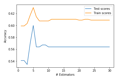
AdaBoost is short for Adaptive Boosting. It is basically a machine learning algorithm that is used as a classifier. Whenever you have a large amount of data and you want divide it into different categories, we need a good classification algorithm to do it. Hence the word ‘boosting’, as in it boosts other algorithms!
scores_test = []
scores_train = []
n_estimators = []for n_est in range(30):
    ada = AdaBoostClassifier(n_estimators = n_est + 1, random_state = 42)
    ada.fit(X_train, y_train)
    n_estimators.append(n_est + 1)
    scores_test.append(ada.score(X_test, y_test))
    scores_train.append(ada.score(X_train, y_train))# Our Ada Boost score on our train set.
ada.score(X_train, y_train)# Our Ada Boost score on our test set.
ada.score(X_test, y_test)
Neural networks are a set of algorithms, modeled loosely after the human brain, that are designed to recognize patterns. They interpret sensory data through a kind of machine perception, labeling or clustering raw input. We can even apply regularization to combat the over fitting issue!
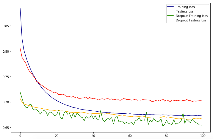
model_dropout = Sequential()n_input = X_train.shape[1]
n_hidden = n_inputmodel_dropout.add(Dense(n_hidden, input_dim = n_input, activation = 'relu'))
model_dropout.add(Dropout(0.5)) # refers to nodes in the first hidden layer
model_dropout.add(Dense(1, activation = 'sigmoid'))model_dropout.compile(loss = 'binary_crossentropy', optimizer = 'adam', metrics = ['acc'])history_dropout = model_dropout.fit(X_train, y_train, validation_data = (X_test, y_test), epochs = 100, batch_size = None)
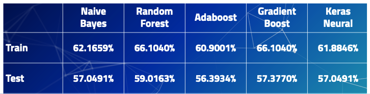
What is this telling us?! Based off of the training score & test score we can see that our model is over fit & is not great at making predictions or analyzing trends. What does it mean that our model is over fit? We have high variance & low bias! High variance can cause an algorithm to model the random noise in the training data, rather than the intended outputs. We still can’t make recommendations off of this since it really doesn’t give us much information!
Second Approach (Natural Language Processing) — The Best Route
My 2nd approach was focusing on the description column. After my 1st approach, I wanted to see how the priority of the attack correlated with what was given in the description. The description column gave us a short explanation of what happened & a suggested FCC compliant resolution in what they might do in stopping that similar event.
In order to better understand the description column, I needed to apply natural language processing (NLP) since computers & statistical models dislike handling text & words. But we can get around this! My approach is similar when cleaning the data & balancing the priorities column, however I have applied some NLP concepts to better understand the description, analyze it, make recommendations & even predict what the next event would be based off of the occurrence of words specific to the events.
Some of the concepts include:
- Pre-processing is the technique of converting raw data into a clean data set.
- Regex, regular expression is a string of text that allows you to create patterns that help match, locate & manage text. Another way to clean the text.
- Lemmatizing is the process of grouping together the inflected forms of a word so they can be analyzed as a single term.
- Stemming is the process of reducing inflected words to their stem, base or root form.
- Countvectorize counts the word frequencies.
- TFIDFVectorizer is the value of a word increases proportionally to count, but is offset by the frequency of the word in the corpus.
Let’s start off by applying regex concepts to our already cleaned data. We also want to strip or clean out common words that are useful but are sporadic in every single description.
# Let's clean the data using Regex.
# Let's use regex to remove the words: service providers, equipment # suppliers, network operators, property managers, public safety
# Let's also remove any mention of any URLs.fcc_csv['Description'] = fcc_csv.Description.map(lambda x: re.sub('\s[\/]?r\/[^s]+', ' ', x))
fcc_csv['Description'] = fcc_csv.Description.map(lambda x: re.sub('http[s]?:\/\/[^\s]*', ' ', x))
fcc_csv['Description'] = fcc_csv.Description.map(lambda x: re.sub('(service providers|equipment suppliers|network operators|property managers|public safety)[s]?', ' ', x,  flags = re.I))
Now that we’ve cleaned our data, we should apply some pre-processing techniques to better understand the words given to use in every description of the event.
# This is a text preprocessing function that gets our data ready for # modeling & creates new columns for the
# description text in their tokenized, lemmatized & stemmed forms.
# This allows for easy selection of
# different forms of the text for use in vectorization & modeling.def preprocessed_columns(dataframe = fcc_csv,
                        column = 'Description',
                        new_lemma_column = 'lemmatized',
                        new_stem_column = 'stemmed',
                        new_token_column = 'tokenized',
                        regular_expression = r'\w+'):

    tokenizer = RegexpTokenizer(regular_expression)
    lemmatizer = WordNetLemmatizer()
    stemmer = PorterStemmer()

    lemmatized = []
    stemmed = []
    tokenized = []


    for i in dataframe[column]:
        tokens = tokenizer.tokenize(i.lower())
        tokenized.append(tokens)        lemma = [lemmatizer.lemmatize(token) for token in tokens]
        lemmatized.append(lemma)                                              stems = [stemmer.stem(token) for token in tokens]
        stemmed.append(stems)

    dataframe[new_token_column] = [' '.join(i) for i in tokenized]
    dataframe[new_lemma_column] = [' '.join(i) for i in lemmatized]
    dataframe[new_stem_column] = [' '.join(i) for i in stemmed]

    return dataframe
We then want to apply countvectorize on our stemmed, lemmatized & tokenized description words in order to control common stop words in the English language, we can do this with the following code. We then can see what the most common words are in the entire data set.
# Instantiate a CountVectorizer removing english stopwords, ngram
# range of unigrams & bigrams.cv = CountVectorizer(stop_words = 'english', ngram_range = (1,2), min_df = 25, max_df = .95)# Create a dataframe of our CV transformed tokenized words
cv_df_token = pd.SparseDataFrame(cv.fit_transform(processed['tokenized']), columns = cv.get_feature_names())
cv_df_token.fillna(0, inplace = True)cv_df_token.head()
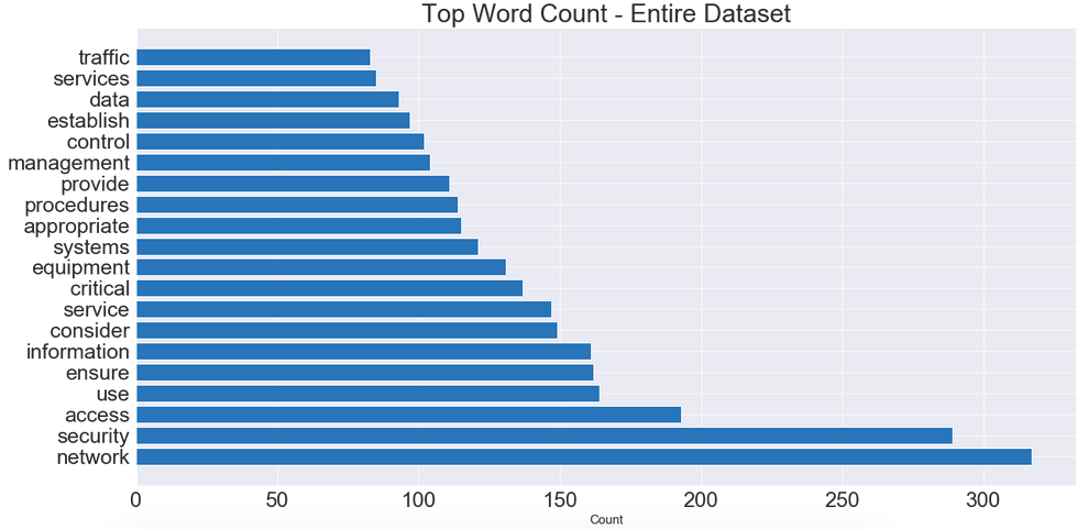
We can see that most of the words that popped up are network or security related. We can use this information to better understand the scope of what these events are! Are the network attacks? Are they network warehouse related? Etc.
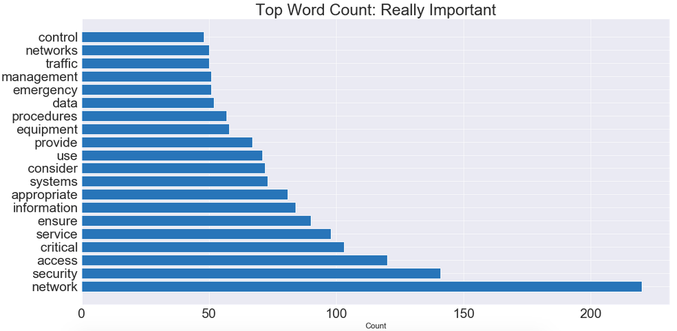
But what if we wanted more information? We can group the descriptions based on the urgency or severity of the importance of the event. Maybe it’s nothing serious so it’s ranked a 0 (Not Important) or really bad ranked as 1 (Really Important). We can do this with the below code based on our pre-processed columns. We can then visualize what the most common really important words are.
# Split our data frame into really "important" & "not important"
# columns.
# We will use the "really_important" descriptions to determine
# severity & to give recommendations/analysis.
fcc_really_important = processed[processed['Priorities'] == 1]
fcc_not_important = processed[processed['Priorities'] == 0]print(fcc_really_important.shape)
print(fcc_not_important.shape)
Finally, we can start modeling regression & classification metrics on the tokenized data. Let’s start by applying a logistic regression model through a pipeline where can apply a grid search tool in order to tune our BEST features or BEST parameters. Let’s establish our X variable, our features! We will use the words or features within the tokenized column within the processed data frame we created above. The processed data frame is an entirely NEW data frame that contains our tokenized, stemmed & lemmatized columns.
Here I decided to focus on the tokenized columns because this specific column functioned the best for parameter tuning & accuracy. To cut on time length for this blog post I decided to focus on the tokenized, what works best, as well! Let’s train-test split it as well.
X_1 = processed['tokenized']# We're train test splitting 3 different columns.
# These columns are the tokenized, lemmatized & stemmed from the
# processed dataframe.
X_1_train, X_1_test, y_train, y_test = train_test_split(X_1, y, test_size = 0.3, stratify = y, random_state = 42)
Now let’s created our pipeline that uses grid search concepts for the best hyper parameters. Once the grid search has fit (this can take awhile!) we can pull out a variety of information and useful objects from the grid search object. Often, we’ll want to apply several transformers to a data set & then finally build a model. If you do all of these steps independently, your code when predicting on test data can be messy. It’ll also be prone to errors. Luckily, we’ll have pipelines!
Here we will be applying a logistic model which can take into consideration LASSO & Ridge penalties.
You should:
- Fit and validate the accuracy of a default logistic regression on the data.
- Perform a gridsearch over different regularization strengths, Lasso & Ridge penalties.
- Compare the accuracy on the test set of your optimized logistic regression to the baseline accuracy & the default model.
- Look at the best parameters found. What was chosen? What does this suggest about our data?
- Look at the (non-zero, if Lasso was selected as best) coefficients & associated predictors for your optimized model. What appears to be the most important predictors?
pipe_cv = Pipeline([
    ('cv', CountVectorizer()),
    ('lr', LogisticRegression())
])params = {
    'lr__C':[0.6, 1, 1.2],
    'lr__penalty':["l1", "l2"],
    'cv__max_features':[None, 750, 1000, 1250],
    'cv__stop_words':['english', None],
    'cv__ngram_range':[(1,1), (1,4)]
}
Now we can apply the pipeline on our logistic regression model within a grid search object. Notice the countvectorize model being instantiated. We did this because we want see how that factors into our accuracy & importance of the words we associated with our network attacks.
# Our Logistic Regression Model.
gs_lr_tokenized_cv = GridSearchCV(pipe_cv, param_grid = params, cv = 5)
gs_lr_tokenized_cv.fit(X_1_train, y_train)
gs_lr_tokenized_cv.score(X_1_train, y_train)gs_lr_tokenized_cv.score(X_1_test, y_test)
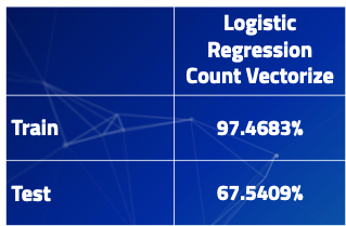
So what can infer from this? Well it looks like we’ve seen a massive increase in model accuracy for a training data as well as 10% increase in accuracy for our testing data. However, the model is still over fit! But still great job! What were our best parameters? We could use this information if we want to tune future logistic models! The below code will show us that!
gs_lr_tokenized_cv.best_params_
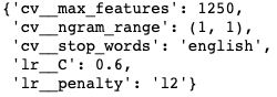
A regression model that uses L1 regularization technique is called Lasso Regression and model which uses L2 is called Ridge Regression. From our best hyper parameters, our models favors a Ridge Regression technique. Now we want to make predictions off of our logistic regression & be able to make suggestions. How do we go upon doing that? Let’s look at the coefficients associated with our features that will predict the outcomes of the best y variable.
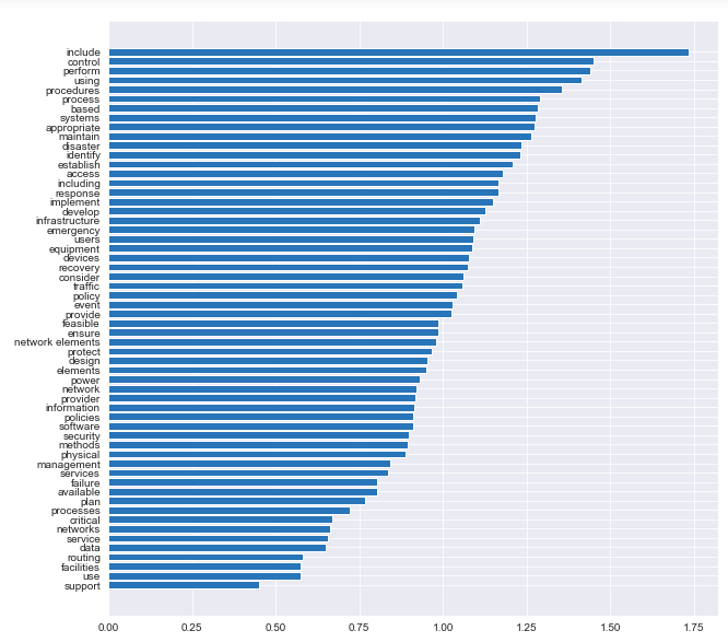
coefs = gs_lr_tokenized_cv.best_estimator_.steps[1][1].coef_
words = pd.DataFrame(zip(cv.get_feature_names(), np.exp(coefs[0])))
words = words.sort_values(1)
Recommendations & Conclusions
Now that I’ve finished modeling & analyzing the data, I can now make suggestions to the FCC as well as any other data scientist or data analyst that plans on doing a project similar to mine.
For future data scientists doing a similar project. Get more data, a better sample of data, increase/decrease complexity of model & regularize. This can help combat the issue of over fitting your data as I experienced through this project. Understand unbalanced classification problems. This can lead to your main direction in solving the problem.
For the FCC’s CSRIC’s best practices, my best recommendation would be to fix the simple issues first so they don’t happen to often & soak up your resources. This can allow them to focus on the more important & complex events or attacks. Based off what I could predict & analyzing the given data.

Simple problems:
- Different Cables
- Color Code Cables
- Better ventilation of warehouse
- Increase power capacity
- Better hardware
- Spacing of antennas

Moderate problems:
- Utilize Network Surveillance
- Provide secure electrical software where feasible
- Find thresholds for new hardware & software
- Virus protection

Complex:
- Minimize single points of failure & software faults
- Device Management Architecture
- Secure networks/encrypted systems
Bio: Aakash Sharma is a Data Scientist, Data Analyst, Cybersecurity Network Engineer, Full Stack Software Developer, and Machine Learning & A.I. Enthusiast.
Original. Reposted with permission.
Related:
- Machine Learning Security
- PySyft and the Emergence of Private Deep Learning
- Top 5 domains Big Data analytics helps to transform