
 Knowing Your Neighbours: Machine Learning on Graphs

 Knowing Your Neighbours: Machine Learning on Graphs
Graph Machine Learning uses the network structure of the underlying data to improve predictive outcomes. Learn how to use this modern machine learning method to solve challenges with connected data.
By Pantelis Elinas, senior machine learning research engineer.
We live in a connected world and generate a vast amount of connected data. Social networks, financial transaction systems, biological networks, transportation systems, and a telecommunication nexus are all examples. The paper citation network displayed in Figure 1 is another example of connected data.

Figure 1: Visualisation of a paper citation network. The nodes represent research papers, while the edges illustrate citations between papers, with the various colour indicative of a report’s subject, with seven colours coding seven topics.
Representing connected data is possible using a graph data structure regularly used in Computer Science.
In this article, we will provide an introduction to the assorted types of connected data, what they represent, and the challenges we can solve. We also introduce graph convolutional networks (GCNs). Using GCN as an example, this paper will also explain how modern machine learning methods can build predictive models of connected data.
Definitions and types of networks
A graph data structure has two basic elements: nodes and edges (see Figure 2 below). Nodes represent entities in the data such as members of an online social network, while edges symbolise relationships between those entities, such as the friendship between members of a social network. This web of nodes and edges form a graph — a mathematical representation of the network structure of the data.
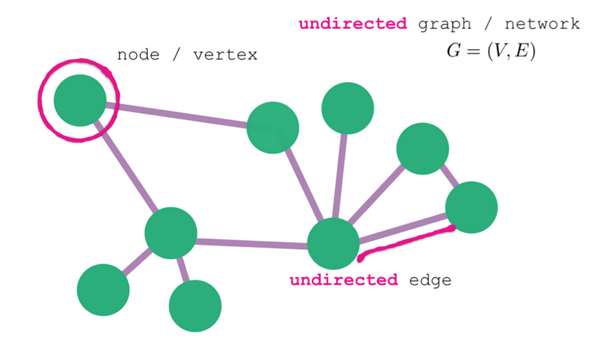
Figure 2: The basic components of a graph (undirected in this case) are nodes and edges.
Graph nodes and edges can optionally have a type. A graph with a single type of node and a single type of edge is called homogeneous. An example of a homogeneous graph is an online social network with nodes representing people and edges representing friendship, where the type of nodes and edges are always the same. On the other hand, a graph with two or more types of node and/or two or more types of edge is called heterogeneous. An online social network with edges of different types says ‘friendship’ and ‘co-worker,’ between nodes of ‘person’ type is an example of a heterogeneous network (see Figure 3 below).

Figure 3: A pictorial representation of two types of graphs, homogeneous (left) and heterogeneous (right). The heterogeneous graph (in black and white) has two different types of nodes, people and cities, that are connected by four different types of edges.
The graph nodes and edges can also incorporate properties called attributes or features. Revisiting the online social network example, a node representing a person, i.e., a person node, may have attributes for their age, salary, hobbies, and location. Similarly, an edge between two people nodes may have a date property establishing when the online relationship began, or a weight property reflective of the strength of the relationship.
We can also classify graphs based on whether they are static or dynamic. True to their name, static graphs do not change with time, while a dynamic graph changes its structure over time, adding and removing nodes and edges, or altering attributes and features (e.g. node attributes can be time series), or both.
What can we learn from graphs?
Given a connected dataset, what kinds of problems can we solve, or put differently, what kinds of queries can we answer? We can broadly classify the kinds of problems connected data can solve into four categories:
- Node Classification
- Link Prediction
- Community Detection
- Graph Classification
There exist other graph problems that don’t necessarily fit in these four categories, e.g., Traveling Salesman Problems. However, for this article, we will focus on the above four categories, as graph machine learning is an excellent tool for solving them.
Node classification, also known as node attribute inference, is the problem of inferring missing or incomplete attribute values of some nodes, given attribute values of other nodes in the network. The advantage over other machine learning methods is that node attribute inference gives you the ability to bring in context and neighbourhood information into your predictions. For example, in an online social network we might be interested in predicting the music preferences of a user’s friendship network (see Figure 4 below).
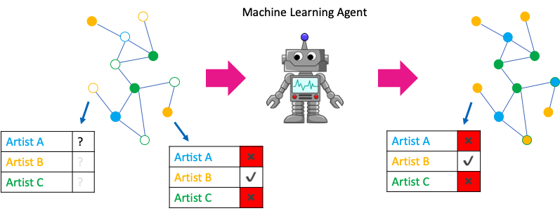
Figure 4: An example node classification problem, inferring an online social network member’s music preferences.
Link prediction, another important problem for network-structured datasets, is the problem of inferring missing or finding hidden relationships between entities. We may be interested in predicting missing relationships because some were hidden from us during data collection. Alternatively, we may be interested in predicting how the network structure will evolve in the future through insertion or deletion of links, given its snapshot at the current time. Link prediction is an algorithm that we use every day, as it is typically the algorithm behind recommender systems. For example, in an online social network, we can use link prediction to suggest new friends to members. Another example is product recommendation for a content provider or an e-commerce website.
Community detection infers communities or clusters of nodes based on the graph’s structure, the similarity of node attributes, or both. There are many applications for community detection, [1]. One example is segmentation of users of a social network into communities based on their hobbies, without having to explicitly ask each user if they are interested in that topic. Instead, answers to topical questions, for example, ‘Do you like fiction or nonfiction?’, are answered by the algorithm using the data gathered from the people the individual frequently interacts with. Such segmentation can be used to deliver targeted ads based on common traits of community members.
Graph classification is the problem of discriminating between graphs of different classes. As an example, consider the representation of a chemical compound as a graph; in this case, nodes are atoms, and edges are bonds between atoms. Given a set of chemical compounds each represented as a graph, we want to predict whether a compound is cancer-hindering or not. This is a graph classification problem, [2].
Node classification example using a Graph Convolutional Network
For the remainder of this article, we’ll demonstrate how to apply graph machine learning to solve a node classification problem in a homogenous graph. In subsequent articles, we will consider state-of-the-art methods for link prediction and community detection.
Our dataset is the paper citation network known as Cora where graph nodes represent research papers, and edges represent citation relationships between the papers. If a paper cites another paper then there is an edge between the two papers. Even though citations are directed, for the purpose of this tutorial, we are going to consider the corresponding edges as undirected.
Each paper has an associated feature vector that encodes information about the vocabulary used in the paper. The feature vector for each paper has 1433 binary elements encoding presence (encoded as 1) or absence (encoded as 0) of 1433 keywords extracted from the entire corpus of the papers’ texts.
Figure 5 demonstrates the Bag-of-Words (BoW) model for two papers in Cora. Each paper also has an attribute representing the subject of the paper. Each paper has one of seven subjects, such as Neural Networks, Probabilistic, Theory, etc. The dataset has 2708 papers (nodes) and 5429 citations (edges).
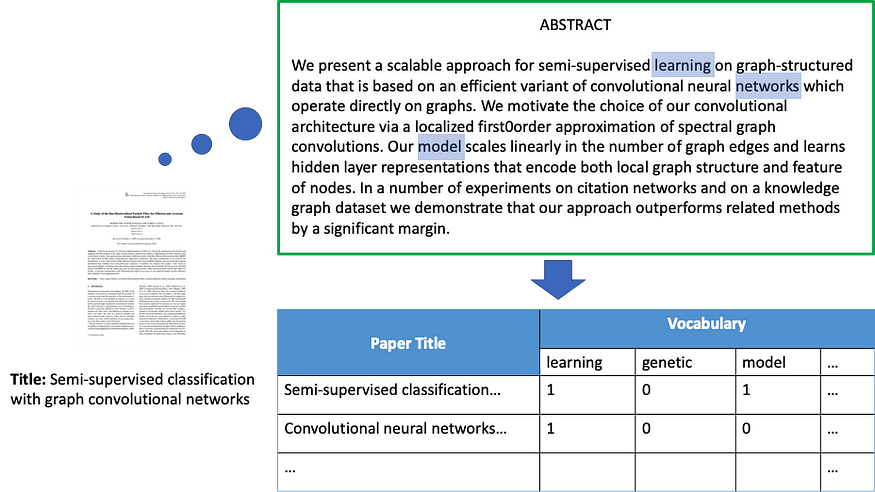
Figure 5: The Bag-of-Words (BoW) features associated with a node in the Cora citation dataset.
Our goal is to train a predictive model to infer the subject of a paper that was hidden from the machine learning algorithm during training. Since subject is categorical with seven categories, this is a multi-class node classification problem.
As a baseline approach, we can use traditional machine learning methods to solve this problem ignoring the relationships between papers. We can stack the nodes’ feature vectors into a 2D array F, known as the design matrix, of dimensionality 2708x1433, and then train a classifier such as Logistic Regression, Neural Network, or Random Forest on a subset of the data. We can use the remaining data for evaluation of the classifier as validation and test sets.
This approach, which captures relationships between the vocabulary used in the papers and their subject, works fairly well. A 2-layer Multi-Layer Perceptron (MLP) trained on only 140 samples (20 training samples per class) has been reported to achieve a test accuracy of approximately 55%, [3].
However, the above method ignores the citation relationships between the papers. We might believe that the relationships provide additional information about the subject of a paper as one would expect that a paper would cite other papers with the same subject. How can we exploit such information?
One approach would be to use manual feature engineering to augment the vocabulary-based feature vectors with graph-related node features. For example, there exists a large amount of literature on methods for calculating quantitative values of the structural position of a node in a graph. A straightforward structural node feature to add would be the number of neighbours a node has in the graph (a node’s degree). Other useful structural node features include PageRank, [4], and various centrality measures. See Figure 6 for some examples of centrality measures.
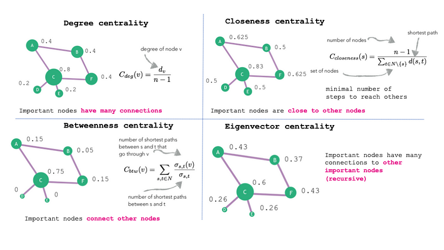
Figure 6: Examples of common centrality measures that can be used for manual feature engineering in graph machine learning.
Manual feature engineering is known to be successful and has been employed extensively over the years. However, what we have learned from the success of deep learning and convolutional neural networks, in particular, is that these algorithms are adept at automatically learning essential features that maximise the performance of a downstream task. Unfortunately, “traditional” neural network and convolutional neural network algorithms cannot directly exploit relationship data.
Despite this, researchers recently proposed graph neural network algorithms that can utilise relationship information in training neural network models on graphs. Of these graph neural network algorithms, Graph Convolutional Network (GCN) [3] is one of the most successful and easy to understand. In this post, we are going to apply a GCN model to our working example of predicting the subject of papers in a citation network. We begin with a brief description of the GCN architecture.
GCN authors introduce a new type of neural network layer known as graph convolutional layer. The architecture of a GCN layer is shown in Figure 7. The layer has trainable parameters: weight matrix W and bias vector b; its inputs are nodes features matrix F, and the normalised graph adjacency matrix A’.
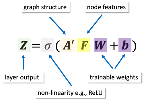
Figure 7: The basic definition of a Graph Convolutional Neural Network (GCN) layer.
The normalised adjacency matrix encodes the graph structure and upon multiplication with the design matrix effectively smooths a node’s feature vector based on those of its immediate neighbours in the graph. A’ is normalised such that each neighbouring node’s contribution is proportional to how connected that node is in the graph.
The layer definition is completed by the application of an element-wise non-linear function, e.g., ReLu, to A’FW+b. The output matrix Z of this layer can be used as input to another GCN layer or any other type of neural network layer, allowing the creation of deep neural architectures able to learn a complex hierarchy of node features needed for the downstream node classification task.
Training a 2-layer GCN model (done in this script using our open-source Python library StellarGraph) with 32 output units per layer on the Cora dataset with just 140 training node labels seen by the model results in a considerable boost in classification accuracy when compared to the baseline 2-layer MLP. Accuracy on predicting the subject of a hold-out test set of papers increases to approximately 81% — an improvement of 21% over the MLP that only uses the BoW node features and ignores citation relationships between the papers. This clearly demonstrates that at least for some datasets utilising relationship information in the data can significantly boost performance in a predictive task.
Node classification is only a small part of graph machine learning but is a very powerful method that can assist in the handling of connected data. If you’d like to know more about graph machine learning, please contact us here, and if you’d like to experiment with node classification or any other graph machine learning algorithms, download our open-source Python library StellarGraph. You can learn more about graph machine learning by studying the StellarGraph demos and ask any questions on our forum!
This work is supported by CSIRO’s Data61, Australia’s leading digital research network.

References:
- Fortunato, S. (2010). “Community detection in graphs,” Physics reports, 486(3–5), 75–174.
- Wale, I. A. Watson, and G. Karypis, “Comparison of descriptor spaces for chemical compound retrieval and classification,” Knowledge and Information Systems, vol. 14, no. 3, pp. 347–375, 2008.
- Kipf, T. N., & Welling, M. (2016). “Semi-supervised classification with graph convolutional networks,” arXiv preprint arXiv:1609.02907.
- Brin, S., & Page, L. (1998). “The anatomy of a large-scale hypertextual web search engine,” Computer networks and ISDN systems, 30(1–7), 107–117.
Bio: Pantelis Elinas is senior machine learning research engineer. He enjoy working on interesting problems, sharing knowledge, and developing useful software tools.
Original. Reposted with permission.
Related: