The 5 Graph Algorithms That Data Scientists Should Know

We as data scientists have gotten quite comfortable with Pandas or SQL or any other relational database.

We are used to seeing our users in rows with their attributes as columns. But does the real world really behave like that?

In a connected world, users cannot be considered as independent entities. They have got certain relationships between each other and we would sometimes like to include such relationships while building our machine learning models.

Now while in a relational database, we cannot use such relations between different rows(users), in a graph database it is fairly trivial to do that.

In this post, I am going to be talking about some of the most important graph algorithms you should know and how to implement them using Python.

Also, here is a Graph Analytics for Big Data course on Coursera by UC San Diego which I highly recommend to learn the basics of graph theory.

1. Connected Components

A graph with 3 connected components

We all know how clustering works?

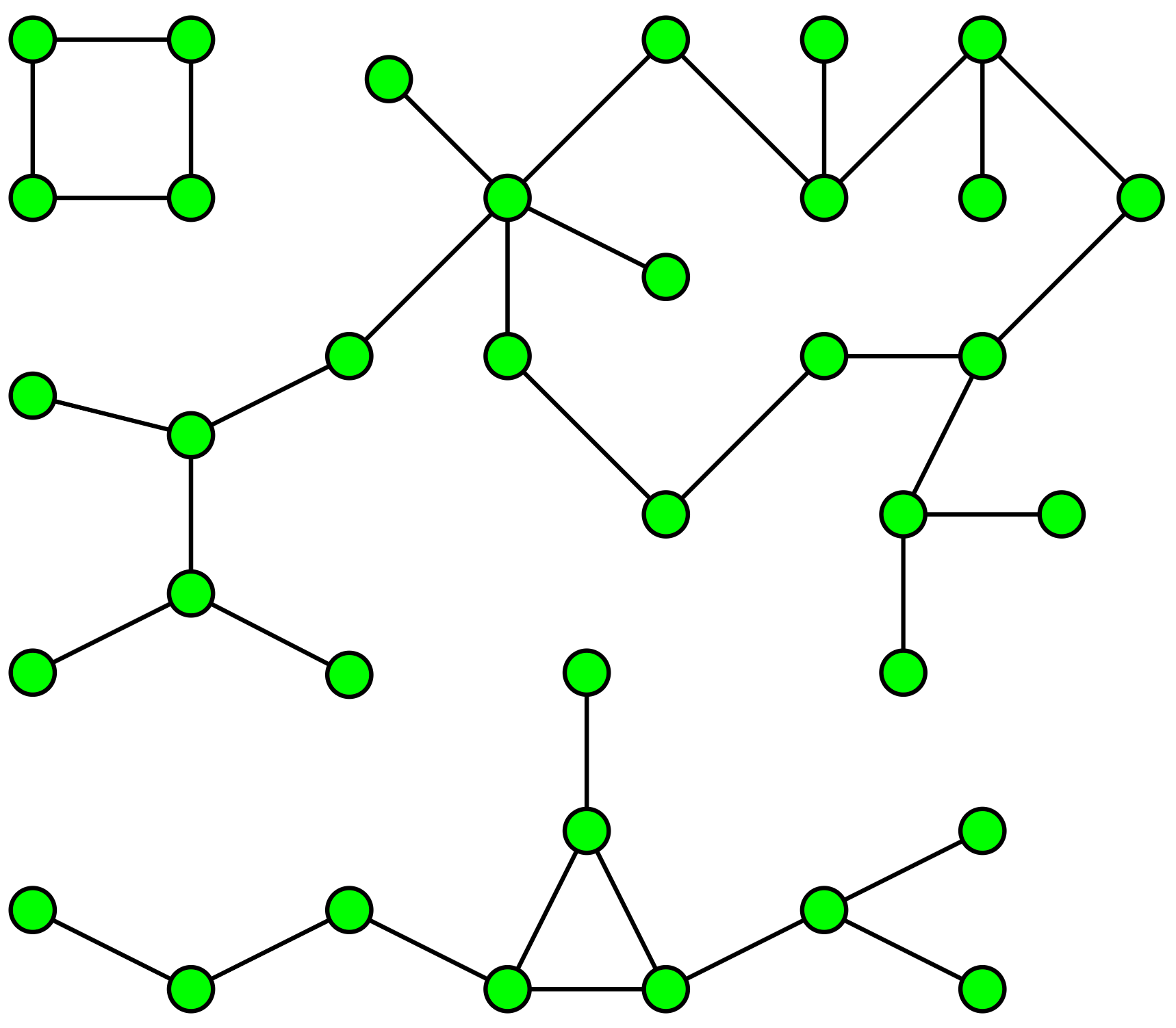
You can think of Connected Components in very layman’s terms as a sort of a hard clustering algorithm which finds clusters/islands in related/connected data.

As a concrete example: Say you have data about roads joining any two cities in the world. And you need to find out all the continents in the world and which city they contain.

How will you achieve that? Come on give some thought.

The connected components algorithm that we use to do this is based on a special case of BFS/DFS. I won’t talk much about how it works here, but we will see how to get the code up and running using Networkx.

Applications

 
From a Retail Perspective: Let us say, we have a lot of customers using a lot of accounts. One way in which we can use the Connected components algorithm is to find out distinct families in our dataset.

We can assume edges(roads) between CustomerIDs based on same credit card usage, or same address or same mobile number, etc. Once we have those connections, we can then run the connected component algorithm on the same to create individual clusters to which we can then assign a family ID.

We can then use these family IDs to provide personalized recommendations based on family needs. We can also use this family ID to fuel our classification algorithms by creating grouped features based on family.

From a Finance Perspective: Another use case would be to capture fraud using these family IDs. If an account has done fraud in the past, it is highly probable that the connected accounts are also susceptible to fraud.

The possibilities are only limited by your own imagination.

Code

 
We will be using the Networkx module in Python for creating and analyzing our graphs.

Let us start with an example graph which we are using for our purpose. Contains cities and distance information between them.

Graph with Some random distances

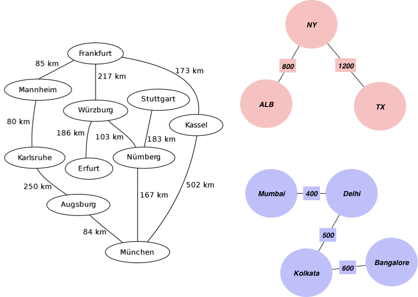
We first start by creating a list of edges along with the distances which we will add as the weight of the edge:

edgelist = [['Mannheim', 'Frankfurt', 85], ['Mannheim', 'Karlsruhe', 80], ['Erfurt', 'Wurzburg', 186], ['Munchen', 'Numberg', 167], ['Munchen', 'Augsburg', 84], ['Munchen', 'Kassel', 502], ['Numberg', 'Stuttgart', 183], ['Numberg', 'Wurzburg', 103], ['Numberg', 'Munchen', 167], ['Stuttgart', 'Numberg', 183], ['Augsburg', 'Munchen', 84], ['Augsburg', 'Karlsruhe', 250], ['Kassel', 'Munchen', 502], ['Kassel', 'Frankfurt', 173], ['Frankfurt', 'Mannheim', 85], ['Frankfurt', 'Wurzburg', 217], ['Frankfurt', 'Kassel', 173], ['Wurzburg', 'Numberg', 103], ['Wurzburg', 'Erfurt', 186], ['Wurzburg', 'Frankfurt', 217], ['Karlsruhe', 'Mannheim', 80], ['Karlsruhe', 'Augsburg', 250],["Mumbai", "Delhi",400],["Delhi", "Kolkata",500],["Kolkata", "Bangalore",600],["TX", "NY",1200],["ALB", "NY",800]]

Let us create a graph using Networkx:

g = nx.Graph()
for edge in edgelist:
    g.add_edge(edge[0],edge[1], weight = edge[2])

Now we want to find out distinct continents and their cities from this graph.

We can now do this using the connected components algorithm as:

for i, x in enumerate(nx.connected_components(g)):
    print("cc"+str(i)+":",x)
------------------------------------------------------------
cc0: {'Frankfurt', 'Kassel', 'Munchen', 'Numberg', 'Erfurt', 'Stuttgart', 'Karlsruhe', 'Wurzburg', 'Mannheim', 'Augsburg'}
cc1: {'Kolkata', 'Bangalore', 'Mumbai', 'Delhi'}
cc2: {'ALB', 'NY', 'TX'}

As you can see we are able to find distinct components in our data. Just by using Edges and Vertices. This algorithm could be run on different data to satisfy any use case that I presented above.

2. Shortest Path

Continuing with the above example only, we are given a graph with the cities of Germany and the respective distance between them.

You want to find out how to go from Frankfurt (The starting node) to Muenchen by covering the shortest distance.

The algorithm that we use for this problem is called Dijkstra. In Dijkstra’s own words:

What is the shortest way to travel from Rotterdam to Groningen, in general: from given city to given city. It is the algorithm for the shortest path, which I designed in about twenty minutes. One morning I was shopping in Amsterdam with my young fiancée, and tired, we sat down on the café terrace to drink a cup of coffee and I was just thinking about whether I could do this, and I then designed the algorithm for the shortest path. As I said, it was a twenty-minute invention. In fact, it was published in ’59, three years later. The publication is still readable, it is, in fact, quite nice. One of the reasons that it is so nice was that I designed it without pencil and paper. I learned later that one of the advantages of designing without pencil and paper is that you are almost forced to avoid all avoidable complexities. Eventually that algorithm became, to my great amazement, one of the cornerstones of my fame.
— Edsger Dijkstra, in an interview with Philip L. Frana, Communications of the ACM, 2001[3]

Applications

• Variations of the Dijkstra algorithm is used extensively in Google Maps to find the shortest routes.
• You are in a Walmart Store. You have different Aisles and distance between all the aisles. You want to provide the shortest pathway to the customer from Aisle A to Aisle D.

• You have seen how LinkedIn shows up 1st-degree connections, 2nd-degree connections. What goes on behind the scenes?

Code

print(nx.shortest_path(g, 'Stuttgart','Frankfurt',weight='weight'))
print(nx.shortest_path_length(g, 'Stuttgart','Frankfurt',weight='weight'))
--------------------------------------------------------
['Stuttgart', 'Numberg', 'Wurzburg', 'Frankfurt']
503

You can also find Shortest paths between all pairs using:

for x in nx.all_pairs_dijkstra_path(g,weight='weight'):
    print(x)
--------------------------------------------------------
('Mannheim', {'Mannheim': ['Mannheim'], 'Frankfurt': ['Mannheim', 'Frankfurt'], 'Karlsruhe': ['Mannheim', 'Karlsruhe'], 'Augsburg': ['Mannheim', 'Karlsruhe', 'Augsburg'], 'Kassel': ['Mannheim', 'Frankfurt', 'Kassel'], 'Wurzburg': ['Mannheim', 'Frankfurt', 'Wurzburg'], 'Munchen': ['Mannheim', 'Karlsruhe', 'Augsburg', 'Munchen'], 'Erfurt': ['Mannheim', 'Frankfurt', 'Wurzburg', 'Erfurt'], 'Numberg': ['Mannheim', 'Frankfurt', 'Wurzburg', 'Numberg'], 'Stuttgart': ['Mannheim', 'Frankfurt', 'Wurzburg', 'Numberg', 'Stuttgart']})('Frankfurt', {'Frankfurt': ['Frankfurt'], 'Mannheim': ['Frankfurt', 'Mannheim'], 'Kassel': ['Frankfurt', 'Kassel'], 'Wurzburg': ['Frankfurt', 'Wurzburg'], 'Karlsruhe': ['Frankfurt', 'Mannheim', 'Karlsruhe'], 'Augsburg': ['Frankfurt', 'Mannheim', 'Karlsruhe', 'Augsburg'], 'Munchen': ['Frankfurt', 'Wurzburg', 'Numberg', 'Munchen'], 'Erfurt': ['Frankfurt', 'Wurzburg', 'Erfurt'], 'Numberg': ['Frankfurt', 'Wurzburg', 'Numberg'], 'Stuttgart': ['Frankfurt', 'Wurzburg', 'Numberg', 'Stuttgart']})....

3. Minimum Spanning Tree

Now we have another problem. We work for a water pipe laying company or an internet fiber company. We need to connect all the cities in the graph we have using the minimum amount of wire/pipe. How do we do this?

An Undirected Graph and its MST on the right.

Applications

• Minimum spanning trees have direct applications in the design of networks, including computer networks, telecommunications networks, transportation networks, water supply networks, and electrical grids (which they were first invented for)
• MST is used for approximating the traveling salesman problem
• Clustering — First construct MST and then determine a threshold value for breaking some edges in the MST using Intercluster distances and Intracluster distances.
• Image Segmentation — It was used for Image segmentation where we first construct an MST on a graph where pixels are nodes and distances between pixels are based on some similarity measure(color, intensity, etc.)

Code

# nx.minimum_spanning_tree(g) returns a instance of type graph
nx.draw_networkx(nx.minimum_spanning_tree(g))

The MST of our graph.

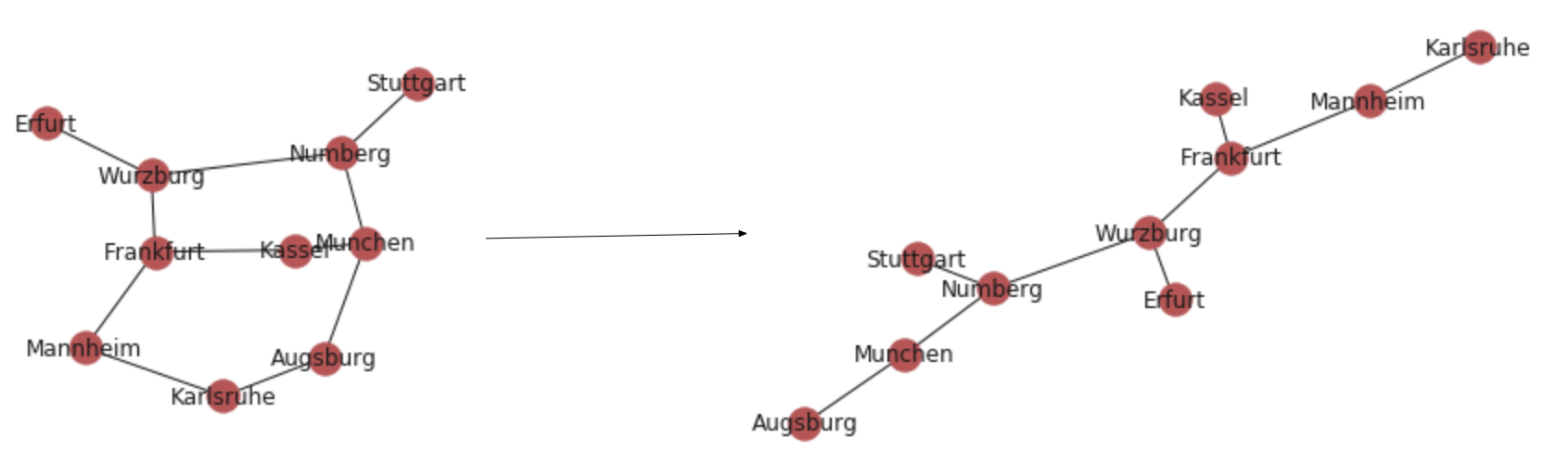
As you can see the above is the wire we gotta lay.

4. Pagerank

This is the page sorting algorithm that powered google for a long time. It assigns scores to pages based on the number and quality of incoming and outgoing links.

Applications

 
Pagerank can be used anywhere where we want to estimate node importance in any network.

• It has been used for finding the most influential papers using citations.
• Has been used by Google to rank pages
• It can be used to rank tweets- User and Tweets as nodes. Create Link between user if user A follows user B and Link between user and Tweets if user tweets/retweets a tweet.
• Recommendation engines

Code

 
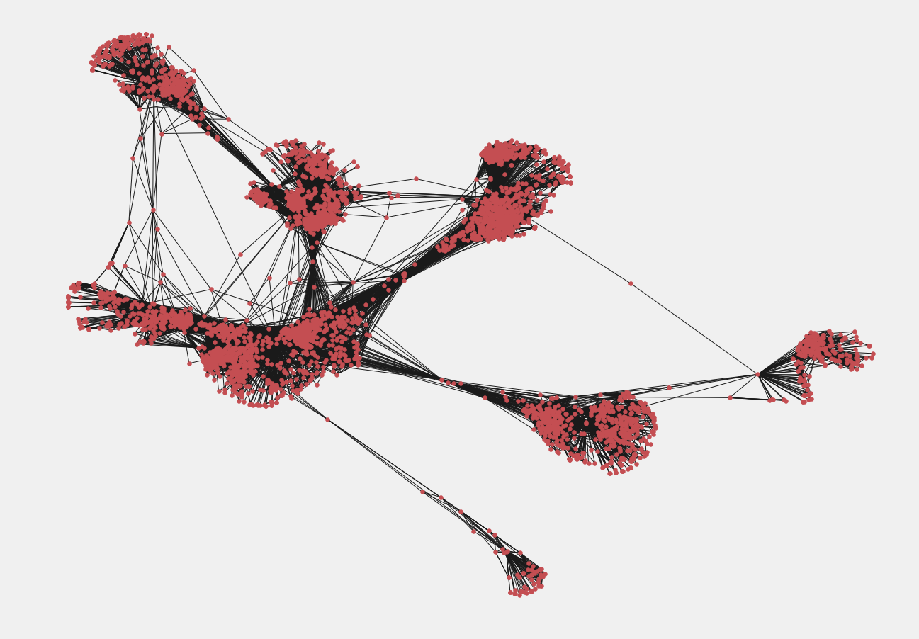
For this exercise, we are going to be using Facebook data. We have a file of edges/links between facebook users. We first create the FB graph using:

# reading the datasetfb = nx.read_edgelist('../input/facebook-combined.txt', create_using = nx.Graph(), nodetype = int)

This is how it looks:

pos = nx.spring_layout(fb)import warnings
warnings.filterwarnings('ignore')plt.style.use('fivethirtyeight')
plt.rcParams['figure.figsize'] = (20, 15)
plt.axis('off')
nx.draw_networkx(fb, pos, with_labels = False, node_size = 35)
plt.show()

FB User Graph

Now we want to find the users having high influence capability.

Intuitively, the Pagerank algorithm will give a higher score to a user who has a lot of friends who in turn have a lot of FB Friends.

pageranks = nx.pagerank(fb)
print(pageranks)
------------------------------------------------------
{0: 0.006289602618466542,
 1: 0.00023590202311540972,
 2: 0.00020310565091694562,
 3: 0.00022552359869430617,
 4: 0.00023849264701222462,
........}

We can get the sorted PageRank or most influential users using:

import operator
sorted_pagerank = sorted(pagerank.items(), key=operator.itemgetter(1),reverse = True)
print(sorted_pagerank)
------------------------------------------------------
[(3437, 0.007614586844749603), (107, 0.006936420955866114), (1684, 0.0063671621383068295), (0, 0.006289602618466542), (1912, 0.0038769716008844974), (348, 0.0023480969727805783), (686, 0.0022193592598000193), (3980, 0.002170323579009993), (414, 0.0018002990470702262), (698, 0.0013171153138368807), (483, 0.0012974283300616082), (3830, 0.0011844348977671688), (376, 0.0009014073664792464), (2047, 0.000841029154597401), (56, 0.0008039024292749443), (25, 0.000800412660519768), (828, 0.0007886905420662135), (322, 0.0007867992190291396),......]

The above IDs are for the most influential users.

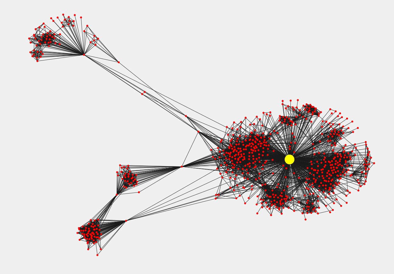
We can see the subgraph for the most influential user:

first_degree_connected_nodes = list(fb.neighbors(3437))
second_degree_connected_nodes = []
for x in first_degree_connected_nodes:
    second_degree_connected_nodes+=list(fb.neighbors(x))
second_degree_connected_nodes.remove(3437)
second_degree_connected_nodes = list(set(second_degree_connected_nodes))subgraph_3437 = nx.subgraph(fb,first_degree_connected_nodes+second_degree_connected_nodes)pos = nx.spring_layout(subgraph_3437)node_color = ['yellow' if v == 3437 else 'red' for v in subgraph_3437]
node_size =  [1000 if v == 3437 else 35 for v in subgraph_3437]
plt.style.use('fivethirtyeight')
plt.rcParams['figure.figsize'] = (20, 15)
plt.axis('off')nx.draw_networkx(subgraph_3437, pos, with_labels = False, node_color=node_color,node_size=node_size )
plt.show()

Our most influential user(Yellow)

5. Centrality Measures

 
There are a lot of centrality measures which you can use as features to your machine learning models. I will talk about two of them. You can look at other measures here.

Betweenness Centrality: It is not only the users who have the most friends that are important, the users who connect one geography to another are also important as that lets users see content from diverse geographies. Betweenness centrality quantifies how many times a particular node comes in the shortest chosen path between two other nodes.

Degree Centrality: It is simply the number of connections for a node.

Applications

 
Centrality measures can be used as a feature in any machine learning model.

Code

 
Here is the code for finding the Betweenness centrality for the subgraph.

pos = nx.spring_layout(subgraph_3437)
betweennessCentrality = nx.betweenness_centrality(subgraph_3437,normalized=True, endpoints=True)node_size =  [v * 10000 for v in betweennessCentrality.values()]
plt.figure(figsize=(20,20))
nx.draw_networkx(subgraph_3437, pos=pos, with_labels=False,
                 node_size=node_size )
plt.axis('off')

You can see the nodes sized by their betweenness centrality values here. They can be thought of as information passers. Breaking any of the nodes with a high betweenness Centrality will break the graph into many parts.

Conclusion

 
In this post, I talked about some of the most influential graph algorithms that have changed the way we live.

With the advent of so much social data, network analysis could help a lot in improving our models and generating value.

And even understanding a little more about the world.

There are a lot of graph algorithms out there, but these are the ones I like the most. Do look into the algorithms in more detail if you like. In this post, I just wanted to get the required breadth into the area.

Let me know if you feel I have left your favorite algorithm in the comments.

Here is the Kaggle Kernel with the whole code.

If you want to read up more on Graph Algorithms here is a Graph Analytics for Big Data course on Coursera by UCSanDiego which I highly recommend to learn the basics of graph theory.

Thanks for the read. I am going to be writing more beginner-friendly posts in the future too. Follow me up at Medium or Subscribe to my blog to be informed about them. As always, I welcome feedback and constructive criticism and can be reached on Twitter @mlwhiz.

 
Bio: Rahul Agarwal is a Data Scientist at Walmart Labs.

Original. Reposted with permission.

Related:

• 10 Great Python Resources for Aspiring Data Scientists
• Coding Random Forests in 100 lines of code*
• Populating a GRAKN.AI Knowledge Graph with the World