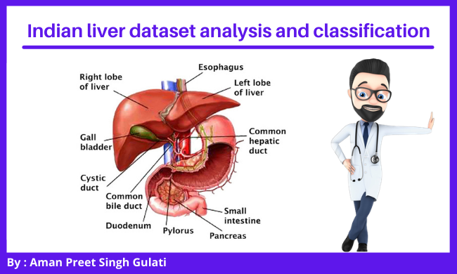
Indian Patient’s Liver Dataset Analysis and Classification
This article was published as a part of the Data Science Blogathon
Purpose
If you google out some basic questions as such:
1. How many liver deaths take place every year in India?
Answer: Liver cirrhosis is the biggest health problem posed by alcohol use, with 1.4 lakh deaths every year.
2. Is liver cirrhosis a lifestyle disease?
Answer: Sadly, no. In fact, it is getting more common in younger people than ever before. Dr. Amrish said that liver disease can set in childhood too as it can pass through genes.
3. Is liver cirrhosis treatable?
Answer: Cirrhosis isn’t curable, but it’s treatable. Alcohol abuse, hepatitis, and fatty liver disease are some of the main causes.
Then you people will get answers like these as I mentioned above, So the purpose and inspiration of this project clearly simplifies the devastating answers from the data available with Google. We do need a system that in some stage reduces the burden on doctors, and today in this article I’ll try to frame a practical logic that will help our healthcare system in a long run.
Content
This data set contains 416 liver patient records and 167 non-liver patient records collected from North East of Andhra Pradesh, India. The “Dataset” column is a class label used to divide groups into a liver patient (liver disease) or not (no disease). This data set contains 441 male patient records and 142 female patient records.
Note: We have not started any data analysis yet, this is just to show you all the authenticity of the dataset.
Acknowledgments
This dataset was downloaded from the UCI ML Repository:
Lichman, M. (2013). UCI Machine Learning Repository.Irvine, CA: the University of California, School of Information and Computer Science.
Problem statement
By using these patient records to determine which patients have liver disease and which ones do not.
Data description
Any patient whose age exceeded 89 is listed as being of age “90”.
Columns:
- Age of the patient
- Gender of the patient
- Total Bilirubin
Bilirubin is an orange-yellow pigment that occurs normally when part of your red blood cells break down. A bilirubin test measures the amount of bilirubin in your blood. It’s used to help find the cause of health conditions like jaundice, anemia, and liver disease.
- Direct Bilirubin
Bilirubin attached by the liver to glucuronic acid, a glucose-derived acid, is called direct or conjugated, bilirubin. Bilirubin not attached to glucuronic acid is called indirect
- Alkaline Phosphatase
Alkaline phosphatase (ALP) is an enzyme in a person’s blood that helps break down proteins. Using an ALP test, it is possible to measure how much of this enzyme is circulating in a person’s blood.
- Alamine Aminotransferase
Alanine aminotransferase (ALT) is an enzyme found primarily in the liver and kidney. ALT is increased with liver damage and is used to screen for and/or monitor liver disease.
- Aspartate Aminotransferase
AST (aspartate aminotransferase) is an enzyme that is found mostly in the liver, but also in muscles. When your liver is damaged, it releases AST into your bloodstream. An AST blood test measures the amount of AST in your blood. The test can help your health care provider diagnose liver damage or disease.
- Total Proteins
Albumin and globulin are two types of protein in your body. The total protein test measures the total amount of albumin and globulin in your body.
- Albumin
- Albumin and Globulin Ratio
“Dataset” field is used to split the data into two sets (patient with liver disease, or no disease).
Alright, then enough of theoretical kinds of stuff let’s get our hands-on building model and,
Let’s get started !
1. Importing Libraries
import pandas as pd
import numpy as np
import matplotlib.pyplot as plt
import seaborn as sns
%matplotlib inline
from sklearn.preprocessing import LabelEncoder
import warnings
warnings.filterwarnings('ignore')
from sklearn.metrics import accuracy_score
from sklearn.model_selection import train_test_split
from sklearn.metrics import classification_report, confusion_matrix
from sklearn import linear_model
from sklearn.linear_model import LogisticRegression
from sklearn.svm import SVC, LinearSVC
from sklearn.ensemble import RandomForestClassifier
from sklearn.naive_bayes import GaussianNB
2. Reading the Data from the CSV file
liver_df = pd.read_csv("indian_liver_patient.csv")
3. Exploratory Data Analysis (EDA)
# Total number of columns in the dataset
liver_df.columns
Output:
Index(['Age', 'Gender', 'Total_Bilirubin', 'Direct_Bilirubin',
       'Alkaline_Phosphotase', 'Alamine_Aminotransferase',
       'Aspartate_Aminotransferase', 'Total_Protiens', 'Albumin',
       'Albumin_and_Globulin_Ratio', 'Dataset'],
      dtype='object')
# Information about the dataset
liver_df.info()
Output:
<class 'pandas.core.frame.DataFrame'>
RangeIndex: 583 entries, 0 to 582
Data columns (total 11 columns):
 #   Column                      Non-Null Count  Dtype
---  ------                      --------------  -----
 0   Age                         583 non-null    int64
 1   Gender                      583 non-null    object
 2   Total_Bilirubin             583 non-null    float64
 3   Direct_Bilirubin            583 non-null    float64
 4   Alkaline_Phosphotase        583 non-null    int64
 5   Alamine_Aminotransferase    583 non-null    int64
 6   Aspartate_Aminotransferase  583 non-null    int64
 7   Total_Protiens              583 non-null    float64
 8   Albumin                     583 non-null    float64
 9   Albumin_and_Globulin_Ratio  579 non-null    float64
 10  Dataset                     583 non-null    int64
dtypes: float64(5), int64(5), object(1)
memory usage: 50.2+ KB
# Checking if there is some null values or not
liver_df.isnull().sum()
Output:
Age                           0
Gender                        0
Total_Bilirubin               0
Direct_Bilirubin              0
Alkaline_Phosphotase          0
Alamine_Aminotransferase      0
Aspartate_Aminotransferase    0
Total_Protiens                0
Albumin                       0
Albumin_and_Globulin_Ratio    4
Dataset                       0
dtype: int64
Inference: We can see there are 4 null values in Albumin_and_Globulin_Ratio.
4. Data Visualization
Inference: We can clearly see in the output as well as in the graph that, it is an imbalanced dataset, any patients diagnosed with liver disease are higher compared to the ones who are not diagnosed.
Inference: We can clearly see in the output as well as in the graph that, number of patient suffering from liver disease are higher in males than in females.
Inference: Here is another interactive plot() that shows, males are at higher risk of chronic liver diseases as compare to females.
Inference: Before, we have seen some of the visualization based on gender (separately), here in this FacetGrid plot we can track cases according to both Gender and Age.
Inference: Here in this plot(), we have plotted Total_bilirubin vs Direct_Bilrubin and got the insight that both of the features have a direct relationship with each other.
Inference: In this FacetGrid plot we are plotting two significant features(Alamine and Aspartate -Aminotransferase) along with Gender as a form of hue and it clearly shows that males are highly effective concerning these two features the most.
Inference: In this plot, we can see that Alkaline _Phosphotase and Alamine_Aminotransferase do have a direct regressive relationship but we can also note that there are a bit “outliers” too from the side of Alamine_Aminotransferase.
Inference: Now with the help of the above plot we can find out that, Total_protiens and Albumin features are in positive regressive nature, with some outliers.
Inference: After plotting Albumin and Albumin_and_Globulin_Ratio we conclude that they both share normal distribution and have a direct relationship like some other features in the dataset.
Inference: Here in this plot, we are trying to show that though Albumin and Globulin Ratio has regressive datapoints yet the most crowded (hotspot) being the male region i.e. they are at high risk in these features too.
We have done enough Data Visualization part by now though you can surely dig deeper in this aspect yet I have covered all the important features in this dataset. As they say,
Visualization act as a campfire around which we gather to tell stories – AI Shalloway
5. Feature engineering
Correlation between all the features
Inference: The 1.00 part of the heatmap signifies that data is positively correlated
6. Splitting data into Train and Test
X_train, X_test, y_train, y_test = train_test_split(X, y, test_size=0.33, random_state=42)
print (X_train.shape)
print (y_train.shape)
print (X_test.shape)
print (y_test.shape)
Output:
(390, 11)
(390,)
(193, 11)
(193,)
7. Model Building
and generalizing from training data, then applying that acquired
knowledge to new data it has never seen before to make predictions and
fulfill its purpose.
a. Logistic Regression
logreg = LogisticRegression()
# Train the model using the training sets and check score
logreg.fit(X_train, y_train)
# Predict Output
log_predicted= logreg.predict(X_test)
logreg_score = round(logreg.score(X_train, y_train) * 100, 2)
logreg_score_test = round(logreg.score(X_test, y_test) * 100, 2)
# Equation coefficient and Intercept
print('Logistic Regression Training Score: n', logreg_score)
print('Logistic Regression Test Score: n', logreg_score_test)
print('Accuracy: n', accuracy_score(y_test,log_predicted))
print('Confusion Matrix: n', confusion_matrix(y_test,log_predicted))
print('Classification Report: n', classification_report(y_test,log_predicted))
Output:
Logistic Regression Training Score:
 70.77
Logistic Regression Test Score:
 72.54
Accuracy:
 0.7253886010362695
Confusion Matrix:
 [[131  10]
 [ 43   9]]
Classification Report:
               precision    recall  f1-score   support

           1       0.75      0.93      0.83       141
           2       0.47      0.17      0.25        52

    accuracy                           0.73       193
   macro avg       0.61      0.55      0.54       193
weighted avg       0.68      0.73      0.68       193
Confusion Matrix
b. Gaussian Naive Bayes
gaussian = GaussianNB()
gaussian.fit(X_train, y_train)
# Predict Output
gauss_predicted = gaussian.predict(X_test)
gauss_score = round(gaussian.score(X_train, y_train) * 100, 2)
gauss_score_test = round(gaussian.score(X_test, y_test) * 100, 2)
print('Gaussian Score: n', gauss_score)
print('Gaussian Test Score: n', gauss_score_test)
print('Accuracy: n', accuracy_score(y_test, gauss_predicted))
print(confusion_matrix(y_test,gauss_predicted))
print(classification_report(y_test,gauss_predicted))
Output:
Gaussian Score:
 53.59
Gaussian Test Score:
 57.51
Accuracy:
 0.5751295336787565
[[60 81]
 [ 1 51]]
              precision    recall  f1-score   support

           1       0.98      0.43      0.59       141
           2       0.39      0.98      0.55        52

    accuracy                           0.58       193
   macro avg       0.68      0.70      0.57       193
weighted avg       0.82      0.58      0.58       193
Confusion Matrix
c. Random Forest
random_forest = RandomForestClassifier(n_estimators=100)
random_forest.fit(X_train, y_train)
# Predict Output
rf_predicted = random_forest.predict(X_test)
random_forest_score = round(random_forest.score(X_train, y_train) * 100, 2)
random_forest_score_test = round(random_forest.score(X_test, y_test) * 100, 2)
print('Random Forest Score: n', random_forest_score)
print('Random Forest Test Score: n', random_forest_score_test)
print('Accuracy: n', accuracy_score(y_test,rf_predicted))
print(confusion_matrix(y_test,rf_predicted))
print(classification_report(y_test,rf_predicted))
Output:
Random Forest Score:
 100.0
Random Forest Test Score:
 71.5
Accuracy:
 0.7150259067357513
[[122  19]
 [ 36  16]]
              precision    recall  f1-score   support

           1       0.77      0.87      0.82       141
           2       0.46      0.31      0.37        52

    accuracy                           0.72       193
   macro avg       0.61      0.59      0.59       193
weighted avg       0.69      0.72      0.70       193
Confusion Matrix
8. Model Evaluation
Conclusion
From the Models (Logistic Regression, Gaussian Naive Bayes, Random Forest) Logistic Regression performs the best on this dataset.
The conclusion of the model also concludes my discussion for today 🙂
Endnotes
Thank you for reading my article 🙂
I hope you have enjoyed the practical implementation and line-by-line explanation of Indian liver dataset analysis and classification using machine learning.
I’m providing the code link here so that you guys can also learn and contribute to this project to make it even better.
You will never want to miss my previous article on, “PAN card fraud detection” published on Analytics Vidhyaas a part of the Data Science Blogathon-9. Refer to this link
Also on, “Drug discovery using machine learning”. Refer to this link.
If got any queries you can connect with me on LinkedIn, refer to this link
About me
Greeting to everyone, I’m currently working as a Data Science Associate Analyst in Zorba Consulting India. Along with part-time work, I’ve got an immense interest in the same field i.e. Data Science along with its other subsets of Artificial Intelligence such as, Computer Vision, Machine learning, and Deep learning feel free to collaborate with me on any project on the above-mentioned domains (LinkedIn).
The media shown in this article are not owned by Analytics Vidhya and are used at the Author’s discretion.


