4 Ways to Handle Insufficient Data In Machine Learning!
This article was published as a part of the Data Science Blogathon
AGENDA:
- Introduction
- Machine Learning pipeline
- Problems with data
- Why do we have insufficient data?
- How it affects the model?
- Overfitting
- Underfitting
- 4 ways to handle insufficient data
- Model Complexity
- Transfer Learning
- Data Augmentation
- Synthetic Data
- References
Introduction
Machine Learning is an interesting area. In the past decade, machine learning has given us self-driving cars, practical speech recognition, effective web search, and a vastly improved understanding of the human genome. Machine learning is so pervasive today that you probably use it dozens of times a day without knowing it. Many researchers also think it is the best way to make progress towards human-level AI.
Source: Google images – Machine Learning
The process of transforming an unstructured data format into a structured one in order to feed it into an ML model is called Data preparation.
Data preparation is the most difficult and time-consuming process while building a machine learning model. There are several actions in data preparation such as dealing with missing data, dropping unnecessary attributes, etc,..the main objective of the data preparation is to fit the data to apply an ML algorithm.
In this blog, we going to dive deeper into the data preparation part of the ml pipeline. we are going to discuss the problems we face with data in the real world and ways to handle insufficient data to get accurate results from the Machine Learning model.
After reading this blog, you will get to know How to process insufficient data efficiently to get accurate results from ML models. We used python language for coding.
Let’s get started!!
What is machine learning?
Machine learning is the scientific study of
algorithms and statistical models that computer systems use to perform a specific task without any instruction, but relying on patterns.
There are 3 types of Machine Learning algorithms:
- Supervised (labeled data)
- Unsupervised (unlabelled data)
- Reinforcement (goal-orientated learning)
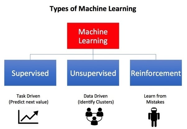
Source: Google Images – Machine Learning Types
Machine Learning helps us to work with,
- Huge amount of data
- Finding patterns from data
- Make intelligent decisions
Machine Learning Pipeline
Now let’s take a quick overview of the Machine Learning pipeline 😀
What is the ML pipeline? Machine Learning Pipeline is also called Machine Learning Workflow. It consists of multiple sequential steps that do everything from data extraction and preprocessing to model training and deployment.

Source: Google Images – ML pipeline
As we all know the data we obtain from the database is unformatted and dirty. So, we just cannot feed the raw dataset into the machine learning model (if done, it leads to inaccurate results). Since the ML model requires well-formatted data to be fed into it, the process of data cleaning is necessary to get accurate predictions from the model.
As we get started by cleaning data, we may encounter many problems like missing values, outliers, and many more. Let us see all the problems associated with data while preparing data for the Machine Learning model.
Problems with data
- Insufficient data
- Too much data
- Non- Representative data
- Missing data
- Duplicate data
- Outliers
So in this blog, we are going to dive deeper into the problem of, insufficient data. As we all know, Data is the new oil and lots of data is generated every minute, second, and microsecond. But one may wonder why do we have insufficient when data is generated in terabytes every day!!
LET’S LOOK AT THE ANSWER 🙂
Why do we have insufficient data?
It is a common struggle in the real world. Nowadays every firm has confidential pieces of information stored in a database that has no access to every employee but some executives. FOR EXAMPLE, in a firm like Healthcare the patient’s information is kept confidential and will not be shared with anyone for privacy reasons. In such cases, we will be provided with a common and small amount of data to make future predictions, which may lead to inaccurate results. Like Healthcare some of the others firms include Consulting, Law, Accounting( Bank services), etc…
Disadvantages:
- Relevant data may not be available.
- The collection process is difficult and time-consuming.
How it affects our Model?
Models trained with this type of data perform poorly while making predictions. It may lead to 2 cases:
1. Over-fitting: Here the training model reads the data too much for too little data. this means the training model actually memorizes the patterns. It has low training errors and high test errors. Does not work well in the real world.
2. Under-fitting:
It builds an overly simple model. This means the data is not trained to our
expectations. the model unable to capture relationship in data. No predictive power.
4 Ways to Handle Insufficient Data
1. Model Complexity:
- Model complexity is nothing but building a simple model with fewer parameters. This method is less susceptible to over-fitting. Example: Naive Bayes, Linear Regression.
- Using Ensemble learning technique: It is defined as several learners are combined to obtain a better performance than any individual learners. It is often used to improve classification and prediction.

Source: Google Images – Ensemble Learning
Implementation:
#Logistic regression
from sklearn.linear_model import LogisticRegression
X_train, X_test, y_train, y_test = train_test_split(X, y, test_size=0.3, random_state=0)
logreg = LogisticRegression()
logreg.fit(X_train, y_train)
y_pred = logreg.predict(X_test)
Voting Ensemble for Classification
from sklearn.linear_model import LogisticRegression
from sklearn.tree import DecisionTreeClassifier
from sklearn.svm import SVC
from sklearn.ensemble import VotingClassifier
kfold = model_selection.KFold(n_splits=10, random_state=seed)
# create the sub models
estimators = []
model1 = LogisticRegression()
estimators.append(('logistic', model1))
model2 = DecisionTreeClassifier()
estimators.append(('cart', model2))
model3 = SVC()
estimators.append(('svm', model3))
# create the ensemble model
ensemble=VotingClassifier(estimators)
results = model_selection.cross_val_score(ensemble, X, Y, cv=kfold)
print(results.mean())
2. Transfer Learning:
- Transfer Learning is used in the case of Deep Learning and
Neural Networks. It uses a pre-built model, which is then tweaked on the small dataset that you have. - It is also defined as the practice of reusing a trained Neural
Networks, that solve a similar problem to yours, usually leaving the network
architecture unchanged and reusing some of the model weights. - It is very much useful when the new dataset is small and
not sufficient to train the model from scratch.
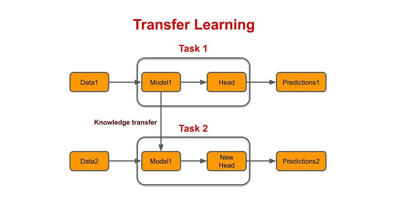
Source: Google Images – Transfer Learning
Interpretation: From the above image, we can clearly see that in Task 1, the Data1 is fed into model and used to make predictions. Then that knowledge is transferred to Task 2 to make another prediction for another dataset( Data2)
Implementation:
STEP 1 – Importing required packages
#Install Tensorflow via PIP using the command below
pip3 install tensorflow==1.13.1
#Install Keras using the command below
pip3 install keras==2.2.4
#Install OpenCV using the command below
pip3 install opencv-python
#Install Numpy using the command below
pip3 install numpy==1.16.1
#Finally, install ImageAI (v2.0.3) using the command below
pip3 install imageai --upgrade
#imported ImageAI training class
from imageai.Prediction.Custom import ModelTraining
#created an instance of the class and set the Model type to ResNet
trainer = ModelTraining()
trainer.setModelTypeAsResNet()
#specified the path to the folder containing dataset (here it is "fruits")
trainer.setDataDirectory("fruits")
#started the training
trainer.trainModel(num_objects=5, num_experiments=50, enhance_data=True, save_full_model=True, batch_size=32, show_network_summary=True, transfer_from_model="resnet50_weights_tf_dim_ordering_tf_kernels.h5", initial_num_objects=1000, transfer_with_full_training=True)
from imageai.Prediction.Custom import CustomImagePrediction
import os
predictor = CustomImagePrediction()
predictor.setModelPath(model_path="transfer_trained_fruits_model_ex-050_acc-0.862500.h5")
predictor.setJsonPath(model_json="model_class.json")
predictor.loadFullModel(num_objects=5)
prediction, probability = predictor.predictImage(image_input=os.path.join(os.getcwd(), "sample.jpg"), result_count=1)
print(prediction, " :", probability)
3. Data Augmentation:
Data Augmentation helps to tweak (make slight improvements) to get new images.
- It takes the pre-existing samples and changes them in some way to
create new samples and also increase the number of training samples and
typically used with Image data. - Disturb images in some way to generate new images, such as,
- Scaling
- Rotation
- Affine Transforms
- These image processing options are often used as pre-processing
techniques to make image classification models built using CNN are robust
Implementation:
# Importing necessary functions
from keras.preprocessing.image import ImageDataGenerator,
array_to_img, img_to_array, load_img
# Initialising the ImageDataGenerator class.
# We will pass in the augmentation parameters in the constructor.
datagen = ImageDataGenerator(
        rotation_range = 40,
        shear_range = 0.2,
        zoom_range = 0.2,
        horizontal_flip = True,
        brightness_range = (0.5, 1.5))
# Loading a sample image
img = load_img('image.jpg')
# Converting the input sample image to an array
x = img_to_array(img)
# Reshaping the input image
x = x.reshape((1, ) + x.shape)
# Generating and saving 5 augmented samples
# using the above defined parameters.
i = 0
for batch in datagen.flow(x, batch_size = 1,
                          save_to_dir ='preview',
                          save_prefix ='image', save_format ='jpeg'):
    i += 1
    if i > 5:
        break
4. Synthetic Data:
- Synthetic
data generally refers to artificially generating samples which
mimic the real-world data (it is one only if we have a good understanding of
features). This may induce bias in existing data.
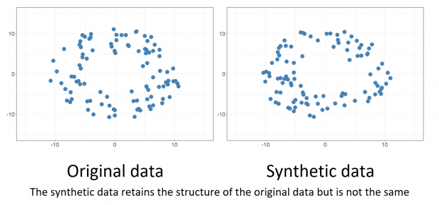
Source: Google Images – Synthetic data
Implementation:
Generating Samples Derived from an Input Dataset
# 1.Get the faces data
# 2.Generate the kernel density model from data
# 3.Use the kernel density to generate new samples of data
#4. Display the original and synthetic faces.
# Fetch the dataset and store in X
faces = dt.fetch_olivetti_faces()
X= faces.data
# Fit a kernel density model using GridSearchCV to determine the best parameter for bandwidth
bandwidth_params = {'bandwidth': np.arange(0.01,1,0.05)}
grid_search = GridSearchCV(KernelDensity(), bandwidth_params)
grid_search.fit(X)
kde = grid_search.best_estimator_
# Generate/sample 8 new faces from this dataset
new_faces = kde.sample(8, random_state=rand_state)
# Show a sample of 8 original face images and 8 generated faces derived from the faces dataset
fig,ax = plt.subplots(nrows=2, ncols=8,figsize=(18,6),subplot_kw=dict(xticks=[], yticks=[]))
for i in np.arange(8):
    ax[0,i].imshow(X[10*i,:].reshape(64,64),cmap=plt.cm.gray)
    ax[1,i].imshow(new_faces[i,:].reshape(64,64),cmap=plt.cm.gray)
ax[0,3].set_title('Original Data',fontsize=20)
ax[1,3].set_title('Synthetic Data',fontsize=20)
fig.subplots_adjust(wspace=.1)
plt.show()
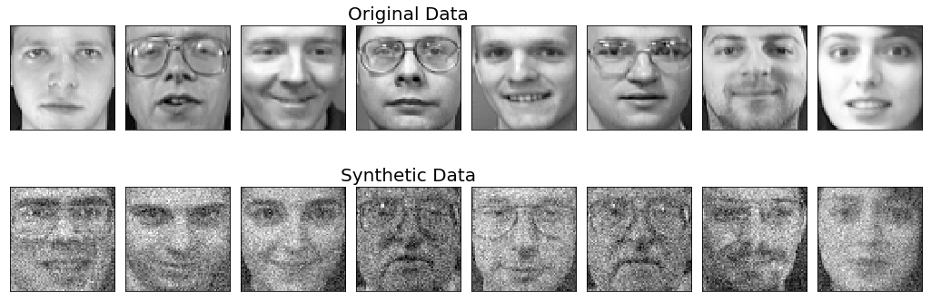
Source: Google Images – Synthetic data (images)
References:
1.https://towardsdatascience.com/building-a-logistic-regression-in-python-step-by-step-becd4d56c9c8
2. https://www.datacamp.com/community/tutorials/ensemble-learning-python
3. https://www.geeksforgeeks.org/python-data-augmentation/
4. https://medium.com/deepquestai/transfer-learning-with-5-lines-of-code-5e69d0290850
Conclusion:
I hope you enjoyed my article and understood how to handle insufficient data in the real world using the above 4 methods which may be very much useful to get a good Machine Learning model.
And I would like to thank Analytics Vidhya for providing me the such a great opportunity to share my knowledge with other people!!
If you have any doubts/suggestions please feel free to contact me on Linkedin / Email.
Once again, THANKS FOR READING :))
About Author:
Hello! This is Priyadharshini, I am currently pursuing M.Sc. in Decision and Computing Sciences. I am very much passionate about Data Science and continuously gaining knowledge from various sources to shine in the Data Science field. I love exploring and analyzing things!!
Thank you!
The media shown in this article are not owned by Analytics Vidhya and are used at the Author’s discretion.


