Analyze Cricket Data With Python : A hands-on guide

This article was published as a part of the Data Science Blogathon

Introduction

Python is a versatile language. It is used for general programming and development purposes, and for complex tasks like Machine Learning, Data Science, and Data Analytics as well. It is not only easy to learn but also has some wonderful libraries, which makes it the first-choice programming language for a lot of people.

In this article, we’ll see one such use case of Python. We will use Python to analyze the performance of Indian cricketer MS Dhoni in his One Day International (ODI) career.

Dataset

If you are familiar with the concept of web scraping, you can scrape the data from this ESPN Cricinfo link. If you are not aware of web scraping, don’t worry! You can directly download the data from here. The data is available as an Excel file to download.

Once you have the dataset with you, you will need to load it in Python. You can use the piece of code below to load the dataset in Python:

Once the dataset has been read, we should look at the head and tail of the dataset to make sure it is imported correctly. The head of the dataset should look like this:

If the data is loaded correctly, we can move on to the next step, data cleaning, and preparation.

Data Cleaning and Preparation

This data has been taken from a webpage, so it is not very clean. We will start by removing the first 2 characters from the opposition string because that is not required.

# removing the first 2 characters in the opposition string
df['opposition'] = df['opposition'].apply(lambda x: x[2:])

Next, we will create a column for the year in which the match was played. Please make sure that the date column is present in the DateTime format in your DataFrame. If not, please use pd.to_datetime() to convert it to DateTime format.

# creating a feature for match year
df['year'] = df['date'].dt.year.astype(int)

We will also create a column indicating whether Dhoni was not out in that innings or not.

# creating a feature for being not out
df['score'] = df['score'].apply(str)
df['not_out'] = np.where(df['score'].str.endswith('*'), 1, 0)

We will now drop the ODI number column because it is not required.

# dropping the odi_number feature because it adds no value to the analysis
df.drop(columns='odi_number', inplace=True)

We will also drop all those matches from our records where Dhoni did not bat, and store this information in a new DataFrame.

# dropping those innings where Dhoni did not bat and storing in a new DataFrame
df_new = df.loc[((df['score'] != 'DNB') & (df['score'] != 'TDNB')), 'runs_scored':]

Finally, we will fix the data types of all the columns present in our new DataFrame.

# fixing the data types of numerical columns
df_new['runs_scored'] = df_new['runs_scored'].astype(int)
df_new['balls_faced'] = df_new['balls_faced'].astype(int)
df_new['strike_rate'] = df_new['strike_rate'].astype(float)
df_new['fours'] = df_new['fours'].astype(int)
df_new['sixes'] = df_new['sixes'].astype(int)

Career Statistics

We will have a look at the descriptive statistics of MS Dhoni’s ODI career. You can use the below code for this:

first_match_date = df['date'].dt.date.min().strftime('%B %d, %Y') # first match
print('First match:', first_match_date)
last_match_date = df['date'].dt.date.max().strftime('%B %d, %Y') # last match
print('nLast match:', last_match_date)
number_of_matches = df.shape[0] # number of mathces played in career
print('nNumber of matches played:', number_of_matches)
number_of_inns = df_new.shape[0] # number of innings
print('nNumber of innings played:', number_of_inns)
not_outs = df_new['not_out'].sum() # number of not outs in career
print('nNot outs:', not_outs)
runs_scored = df_new['runs_scored'].sum() # runs scored in career
print('nRuns scored in career:', runs_scored)
balls_faced = df_new['balls_faced'].sum() # balls faced in career
print('nBalls faced in career:', balls_faced)
career_sr = (runs_scored / balls_faced)*100 # career strike rate
print('nCareer strike rate: {:.2f}'.format(career_sr))
career_avg = (runs_scored / (number_of_inns - not_outs)) # career average
print('nCareer average: {:.2f}'.format(career_avg))
highest_score_date = df_new.loc[df_new.runs_scored == df_new.runs_scored.max(), 'date'].values[0]
highest_score = df.loc[df.date == highest_score_date, 'score'].values[0] # highest score
print('nHighest score in career:', highest_score)
hundreds = df_new.loc[df_new['runs_scored'] >= 100].shape[0] # number of 100s
print('nNumber of 100s:', hundreds)
fifties = df_new.loc[(df_new['runs_scored']>=50)&(df_new['runs_scored']<100)].shape[0] #number of 50s
print('nNumber of 50s:', fifties)
fours = df_new['fours'].sum() # number of fours in career
print('nNumber of 4s:', fours)
sixes = df_new['sixes'].sum() # number of sixes in career
print('nNumber of 6s:', sixes)

The output should look like this:

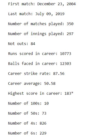
This gives us a good glimpse of MS Dhoni’s overall career. He started playing in 2004, and last played an ODI in 2019. In a career spanning over 15 years, he has scored 10 hundred and an astonishing 73 fifties. He has scored over 10,000 runs in his career at an average of 50.6 and a strike rate of 87.6. His highest score is 183*.

We will now do a more thorough analysis of his performance against different teams. We will also look at his year-on-year performance. We will take the help of visualizations for this.

Analysis

Firstly, we will look at how many matches he has played against different oppositions. You can use the following piece of code for this purpose:

# number of matches played against different oppositions
df['opposition'].value_counts().plot(kind='bar', title='Number of matches against different oppositions', figsize=(8, 5));

The output should look like this:

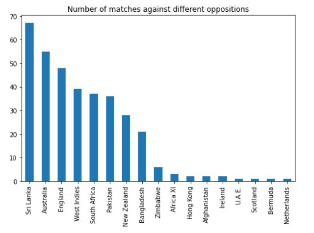
We can see that he has played the majority of his matches against Sri Lanka, Australia, England, West Indies, South Africa, and Pakistan.

Let us look at how many runs he has scored against different oppositions. You can use the following code snippet to generate the result:

runs_scored_by_opposition = pd.DataFrame(df_new.groupby('opposition')['runs_scored'].sum())
runs_scored_by_opposition.plot(kind='bar', title='Runs scored against different oppositions', figsize=(8, 5))
plt.xlabel(None);

The output will look like this:

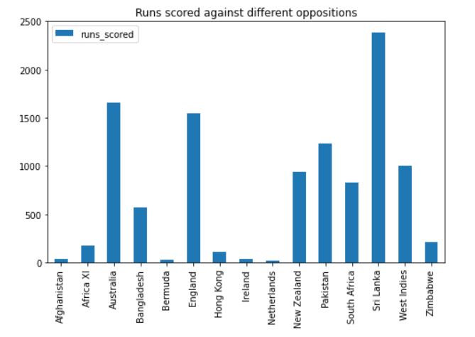
We can see that Dhoni has scored the most runs against Sri Lanka, followed by Australia, England, and Pakistan. He has also played a lot of matches against these teams, so it makes sense.

To get a clearer picture, let us look at his batting average against each team. The following piece of code will help us with getting the desired result:

innings_by_opposition = pd.DataFrame(df_new.groupby('opposition')['date'].count())
not_outs_by_opposition = pd.DataFrame(df_new.groupby('opposition')['not_out'].sum())
temp = runs_scored_by_opposition.merge(innings_by_opposition, left_index=True, right_index=True)
average_by_opposition = temp.merge(not_outs_by_opposition, left_index=True, right_index=True)
average_by_opposition.rename(columns = {'date': 'innings'}, inplace=True)
average_by_opposition['eff_num_of_inns'] = average_by_opposition['innings'] - average_by_opposition['not_out']
average_by_opposition['average'] = average_by_opposition['runs_scored'] / average_by_opposition['eff_num_of_inns']
average_by_opposition.replace(np.inf, np.nan, inplace=True)
major_nations = ['Australia', 'England', 'New Zealand', 'Pakistan', 'South Africa', 'Sri Lanka', 'West Indies']

For generating the plot, use the code snippet below:

plt.figure(figsize = (8, 5))
plt.plot(average_by_opposition.loc[major_nations, 'average'].values, marker='o')
plt.plot([career_avg]*len(major_nations), '--')
plt.title('Average against major teams')
plt.xticks(range(0, 7), major_nations)
plt.ylim(20, 70)
plt.legend(['Avg against opposition', 'Career average']);

The output will look like this:

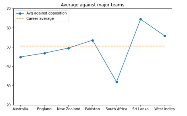
As we can see, Dhoni has performed remarkably against tough teams like Australia, England, and Sri Lanka. His average against these teams is either close to his career average, or slightly higher. The only team against whom he has not performed well is South Africa.

Let us now look at his year-on-year statistics. We will start by looking at how many matches he has played each year after his debut. The code for that will be:

df['year'].value_counts().sort_index().plot(kind='bar', title='Matches played by year', figsize=(8, 5))
plt.xticks(rotation=0);

The plot will look like this:

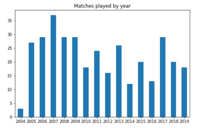
We can see that in 2012, 2014, and 2016, Dhoni played very few ODI matches for India. Overall, after 2005-2009, the average number of matches he played reduced slightly.

We should also look at how many runs he has scored every year. The code for that will be:

df_new.groupby('year')['runs_scored'].sum().plot(kind='line', marker='o', title='Runs scored by year', figsize=(8, 5))
years = df['year'].unique().tolist()
plt.xticks(years)
plt.xlabel(None);

The output should look like this:

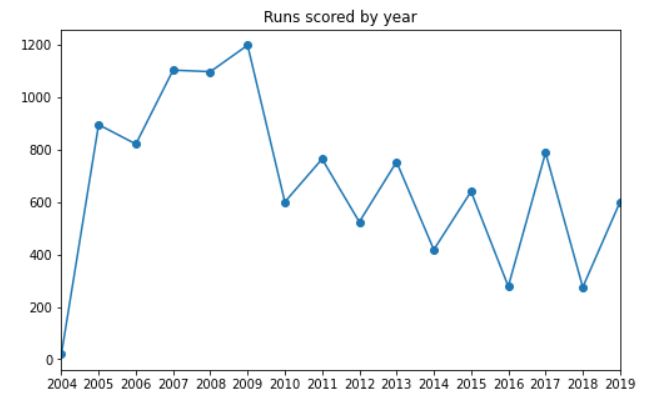
It can be clearly seen that Dhoni scored the most runs in the year 2009, followed by 2007 and 2008. The number of runs started reducing post-2010 (because the number of matches played also started reducing).

Finally, let’s look at his career batting average progression by innings. This is time-series data and has been plotted on a line plot. The code for that will be:

df_new.reset_index(drop=True, inplace=True)
career_average = pd.DataFrame()
career_average['runs_scored_in_career'] = df_new['runs_scored'].cumsum()
career_average['innings'] = df_new.index.tolist()
career_average['innings'] = career_average['innings'].apply(lambda x: x+1)
career_average['not_outs_in_career'] = df_new['not_out'].cumsum()
career_average['eff_num_of_inns'] = career_average['innings'] - career_average['not_outs_in_career']
career_average['average'] = career_average['runs_scored_in_career'] / career_average['eff_num_of_inns']

The code snippet for the plot will be:

plt.figure(figsize = (8, 5))
plt.plot(career_average['average'])
plt.plot([career_avg]*career_average.shape[0], '--')
plt.title('Career average progression by innings')
plt.xlabel('Number of innings')
plt.legend(['Avg progression', 'Career average']);

The output plot will look like this:

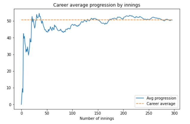
We can see that after a slow start and a dip in performance around innings number 50, Dhoni’s performance picked up substantially. Towards the end of his career, he consistently averaged above 50.

EndNote

In this article, we looked at the batting performance of Indian cricketer MS Dhoni. We looked at his overall career stats, his performance against different oppositions, and his year-on-year performance.

This article has been written by Vishesh Arora. You can connect with me on LinkedIn.

The media shown in this article are not owned by Analytics Vidhya and are used at the Author’s discretion.

Vishesh Arora 23 Sep 2022