Brain Tumor Detection and Localization using Deep Learning: Part 2
Problem Statement:
To predict and localize brain tumors through image segmentation from the MRI dataset available in Kaggle.
This is the second part of the series. If you don’t have yet read the first part, I recommend visiting Brain Tumor Detection and Localization using Deep Learning: Part 1 to better understand the code as both parts are interrelated.
We have trained a classification model on top of ResNet50 which classifies whether a brain MRI has a tumor or not using callbacks to increase our performance. In this part, we will train a model to localize tumor using image segmentation.
Prerequisite:
Deep Learning
Now, let us head towards the implementation of the second part i.e, Building a segmentation model to localize tumors.
The goal of image segmentation is to understand the image at the pixel level. It associates each pixel with a certain class. The output produced by the image segmentation model is called the mask of the image.
- First of all, select the records which have the mask value of 1 from the data frame we created in the last part because we can only localize the tumor if it exists.
# Get the dataframe containing MRIs which have masks associated with them.
brain_df_mask = brain_df[brain_df['mask'] == 1]
brain_df_mask.shape
Output: (1373, 4)
- Split the data into train and test datasets. Here first, we split the whole data into train and validation and further we split half of the validation data into test data.
from sklearn.model_selection import train_test_split
X_train, X_val = train_test_split(brain_df_mask, test_size=0.15)
X_test, X_val = train_test_split(X_val, test_size=0.5)
- We will again generate dummy data i.e, training_generator and validation_generator using DataGenerator. For this purpose, we will first create a list of the image and mask path to pass into the generator.
train_ids = list(X_train.image_path)
train_mask = list(X_train.mask_path)

val_ids = list(X_val.image_path)
val_mask= list(X_val.mask_path)

# Utilities file contains the code for custom data generator
from utilities import DataGenerator

# create image generators
training_generator = DataGenerator(train_ids,train_mask)
validation_generator = DataGenerator(val_ids,val_mask)
- Define a method Resblock as shown below to use in our deep learning model.
The Resblocks are used in the model to get better results. These blocks are simply a bunch of layers. The main eccentricity of the resblocks is that a residual function is learned on the top and information is passed along the bottom unchanged.
def resblock(X, f):

  # make a copy of input
  X_copy = X

  X = Conv2D(f, kernel_size = (1,1) ,strides = (1,1),kernel_initializer ='he_normal')(X)
  X = BatchNormalization()(X)
  X = Activation('relu')(X)

  X = Conv2D(f, kernel_size = (3,3), strides =(1,1), padding = 'same', kernel_initializer ='he_normal')(X)
  X = BatchNormalization()(X)

  X_copy = Conv2D(f, kernel_size = (1,1), strides =(1,1), kernel_initializer ='he_normal')(X_copy)
  X_copy = BatchNormalization()(X_copy)

  # Adding the output from main path and short path together
  X = Add()([X,X_copy])
  X = Activation('relu')(X)

  return X
- Similarly, define the upsample_concat method that upscale and concatenate the values passed. The Upsampling layer is a simple layer with no weights that will double the dimensions of input.
def upsample_concat(x, skip):
  x = UpSampling2D((2,2))(x)
  merge = Concatenate()([x, skip])

  return merge
- Build a segmentation model adding below shown layers including the above-defined resblock and upsample_concat.
input_shape = (256,256,3)

# Input tensor shape
X_input = Input(input_shape)

# Stage 1
conv1_in = Conv2D(16,3,activation= 'relu', padding = 'same', kernel_initializer ='he_normal')(X_input)
conv1_in = BatchNormalization()(conv1_in)
conv1_in = Conv2D(16,3,activation= 'relu', padding = 'same', kernel_initializer ='he_normal')(conv1_in)
conv1_in = BatchNormalization()(conv1_in)
pool_1 = MaxPool2D(pool_size = (2,2))(conv1_in)

# Stage 2
conv2_in = resblock(pool_1, 32)
pool_2 = MaxPool2D(pool_size = (2,2))(conv2_in)

# Stage 3
conv3_in = resblock(pool_2, 64)
pool_3 = MaxPool2D(pool_size = (2,2))(conv3_in)

# Stage 4
conv4_in = resblock(pool_3, 128)
pool_4 = MaxPool2D(pool_size = (2,2))(conv4_in)

# Stage 5 (Bottle Neck)
conv5_in = resblock(pool_4, 256)

# Upscale stage 1
up_1 = upsample_concat(conv5_in, conv4_in)
up_1 = resblock(up_1, 128)

# Upscale stage 2
up_2 = upsample_concat(up_1, conv3_in)
up_2 = resblock(up_2, 64)

# Upscale stage 3
up_3 = upsample_concat(up_2, conv2_in)
up_3 = resblock(up_3, 32)

# Upscale stage 4
up_4 = upsample_concat(up_3, conv1_in)
up_4 = resblock(up_4, 16)

# Final Output
output = Conv2D(1, (1,1), padding = "same", activation = "sigmoid")(up_4)

model_seg = Model(inputs = X_input, outputs = output )
- Compile the model trained above. This time we will customize the parameters of the optimizer. Focal tversky is the loss function and tversky is the measure.
# Utilities file also contains the code for custom loss function
from utilities import focal_tversky, tversky

# Compile the model
adam = tf.keras.optimizers.Adam(lr = 0.05, epsilon = 0.1)
model_seg.compile(optimizer = adam, loss = focal_tversky, metrics = [tversky])
- Now, you know the callbacks that we used in our classifier model. We will use the same to get better performance. Finally, we train our segmentation model.
# use early stopping to exit training if validation loss is not decreasing even after certain epochs.
earlystopping = EarlyStopping(monitor='val_loss', mode='min', verbose=1, patience=20)

# save the best model with lower validation loss
checkpointer = ModelCheckpoint(filepath="ResUNet-weights.hdf5", verbose=1, save_best_only=True)

model_seg.fit(training_generator, epochs = 1, validation_data = validation_generator, callbacks = [checkpointer, earlystopping])
- Predict the mask for our test dataset. Here, the model is the classifier model trained in the earlier part and model_seg is the segmentation model trained above.
from utilities import prediction

# making prediction
image_id, mask, has_mask = prediction(test, model, model_seg)
The output will give us the image path, predicted mask, and the class label.
- Creating a data frame from the predicted result and merge with the test data frame on the image_path.
# creating a dataframe for the result
df_pred = pd.DataFrame({'image_path': image_id,'predicted_mask': mask,'has_mask': has_mask})

# Merge the dataframe containing predicted results with the original test data.
df_pred = test.merge(df_pred, on = 'image_path')
df_pred.head()
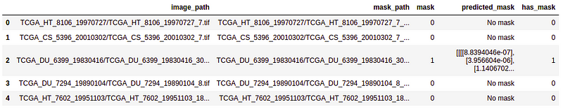
As you can see in the output, we have now our final predicted mask merged in our data frame.
- Finally, visualize the original image, original mask, and predicted mask all together to analyze the accuracy of our segmentation model.
count = 0
fig, axs = plt.subplots(10, 5, figsize=(30, 50))
for i in range(len(df_pred)):
  if df_pred['has_mask'][i] == 1 and count < 5:
    # read the images and convert them to RGB format
    img = io.imread(df_pred.image_path[i])
    img = cv2.cvtColor(img, cv2.COLOR_BGR2RGB)
    axs[count][0].title.set_text("Brain MRI")
    axs[count][0].imshow(img)

    # Obtain the mask for the image
    mask = io.imread(df_pred.mask_path[i])
    axs[count][1].title.set_text("Original Mask")
    axs[count][1].imshow(mask)

    # Obtain the predicted mask for the image
    predicted_mask = np.asarray(df_pred.predicted_mask[i])[0].squeeze().round()
    axs[count][2].title.set_text("AI Predicted Mask")
    axs[count][2].imshow(predicted_mask)

    # Apply the mask to the image 'mask==255'
    img[mask == 255] = (255, 0, 0)
    axs[count][3].title.set_text("MRI with Original Mask (Ground Truth)")
    axs[count][3].imshow(img)

    img_ = io.imread(df_pred.image_path[i])
    img_ = cv2.cvtColor(img_, cv2.COLOR_BGR2RGB)
    img_[predicted_mask == 1] = (0, 255, 0)
    axs[count][4].title.set_text("MRI with AI Predicted Mask")
    axs[count][4].imshow(img_)
    count += 1

fig.tight_layout()
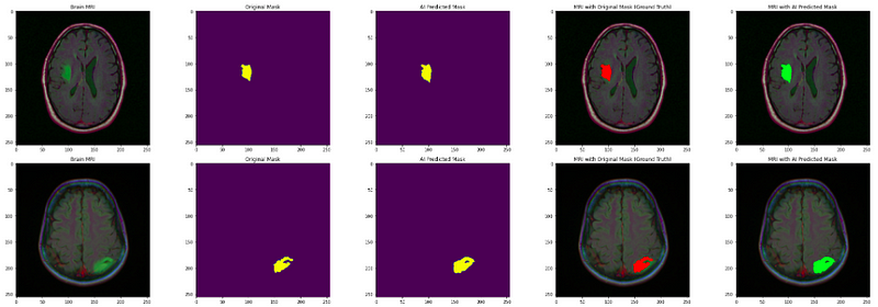
The output shows that our segmentation model localizes the tumor really well. Well done!
Further, you can try adding more layers to the models trained so far and analyze the performance. Also, you can apply similar solutions to other problem statements as image segmentation is an area of great interest nowadays. Don’t forget to share your solutions with us!
Being a Data Science enthusiast, I write similar articles related to Machine Learning, Deep Learning, Computer Vision, and many more.
Your suggestions and doubts are welcomed here in the comment section. Thank you for reading my article!


where is utilities file?? please share the utilities file.
how can we get utilities