A Guide to Machine Learning Pipelines and Orchest

Image 1
Introduction
In this guide, we will learn the importance of Machine Learning (ML) pipelines and how to install and use the Orchest platform. We will be also using Natural Language Processing beginner problem from Kaggle by classifying tweets into disaster and non-disaster tweets. The ML pipelines are independently executable code to run multiple tasks which include data preparation and training machine learning models. The figure below shows how each step has a specific role and how tracking those steps are easy. Azure Machine Learning
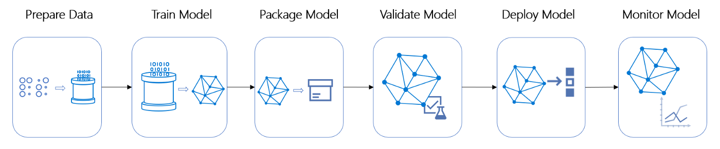 Image 2
Why use Pipelines?
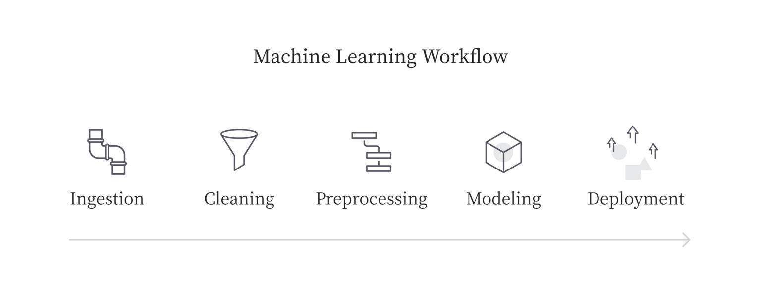
Image 3
The problems arise where you have to deploy these models into production. You need flexibility in scaling your system, tracking the changes, and maintaining similar versions in the entire ecosystem.
- Volume: when deploying multiple versions of models, you need to run a similar workflow with few changes in hyperparameters, data post-processing, or removing additional steps. Pipelines provide flexibility and reproducibility of experiments.
- Variety: when adding additional processes to your workflow, copy-pasting is the bad approach.
- Versioning: When you want to make changes in a commonly used part of your workflow, you have to manually make changes in each workflow if you are not using pipelines. That can create room for error and it’s not efficient. The ML pipeline and why it’s important | Algorithmia Blog
What is Orchest?
Orchest is a data pipeline ecosystem that does not requires DAGs or any third-party integration. The environment is simple to navigate, and you get to use your favorite IDE Jupiter Lab and VSCode. You can also code your steps in various languages such as Python, R, and Julia.
A pipeline in Orchest contains steps. The individual steps are executable files that execute within the isolated environment, and they are connected via nodes that define data flow from one step to another. The Orchest environment is user-friendly so that you can pick and drop steps and easily connect them with multiple steps. It also allows you to visualize the progress and helps you in debugging the code. You can watch the video below to understand it better.
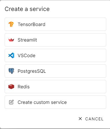
Additional Service
Scheduling Pipeline
Installing Orchest
In this section, we will learn how to install the Orchest on your PC with simple steps. If you are using Linux operating system, then you have to write one line of code. Make sure you have the latest Docker Desktop installed in your system.
Windows
Follow the steps below to install the platform successfully and for more information check Installation (orchest.readthedocs.io)
- Docker Engine latest version: run
docker versionto check. - Docker must be configured to use WSL 2.
- Ubuntu 20.04 LTS for Windows.
- Run the script below inside the Ubuntu environment.
Linux
Just copy and paste the code below in the command line and press enter.
git clone https://github.com/orchest/orchest.git && cd orchest
./orchest install

# Verify the installation.
./orchest version --ext

# Start Orchest.
./orchest start
Orchest Cloud
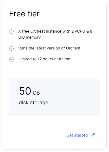
If you are going to use Orchest cloud, you can sign up for free tire and start working on your project without installing anything https://cloud.orchest.io/signup.
Disaster Tweets Project
This challenge is perfect for data scientists looking to get started with Natural Language Processing. Natural Language Processing with Disaster Tweets | Kaggle. You will be predicting whether a tweet is about a real disaster (1) or not (0).
Files
- train.csv – the training set
- test.csv – the test set
- sample_submission.csv – a sample submission file in the correct format
Columns
id– a unique identifier for each tweettext– the text of the tweetlocation– the location the tweet was sent from (may be blank)keyword– a particular keyword from the tweet (may be blank)target– in train.csv only, real disaster tweet (1) or not (0)
Initialize
After the account signup, you will see the project tab where you can click on the add projects tab.
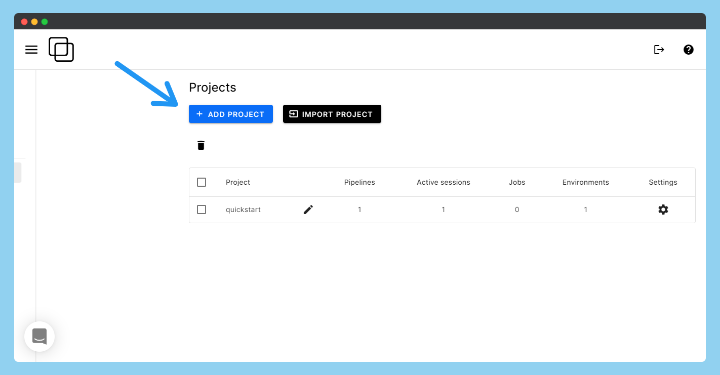
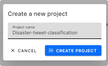
Write preferred project name and press create project button.
You now need to create a pipeline and start working on the project. A single project can have multiple pipelines.
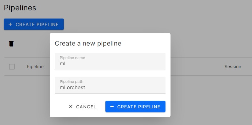
We have finally reached a blank canvas with multiple options to get started. The next step is to add steps to our pipeline.
Adding Steps
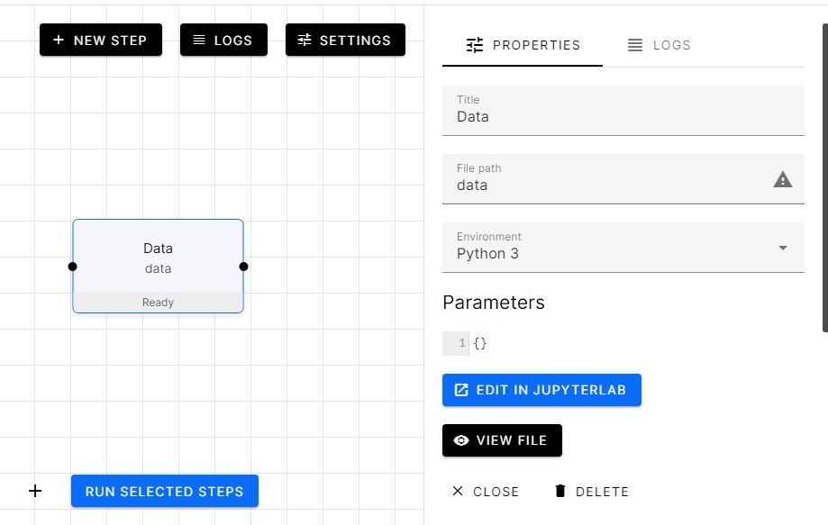
Press on the New Step button and then add the tile for your step. In our case, it’s “Data”. The warning sign says that the data file doesn’t exist. You can click on the warning sign and create either a .ipynb or .py file.
Jupyter Lab
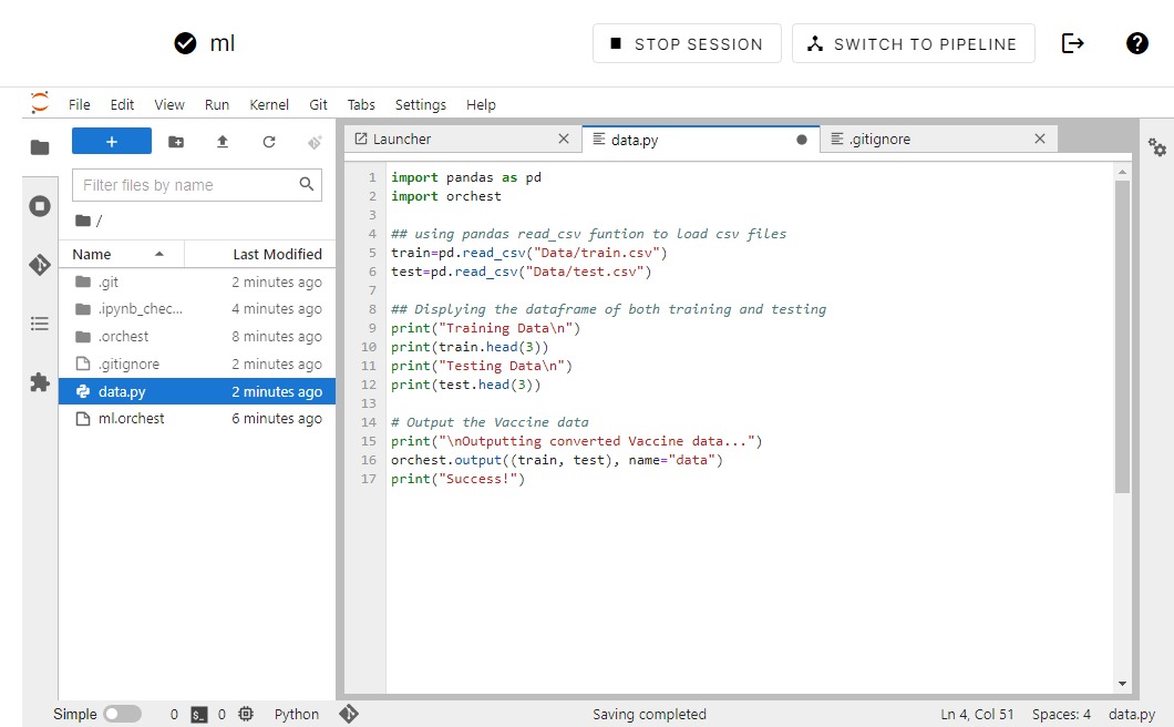
- Importing train and test CSV files
- Display the first three samples of each dataframe
- forwarding data by using the orchest library.
- To export data, use orchest.output((variable1, variable2, …), name = )
- To Import data, first create object: data=orchest.get_inputs() then variable1, variable2, …= data [“”]
import pandas as pd
import orchest
## using pandas read_csv funtion to load csv files
train=pd.read_csv("Data/train.csv")
test=pd.read_csv("Data/test.csv")
## Displying the dataframe of both training and testing
print("Training Datan")
print(train.head(3))
print("Testing Datan")
print(test.head(3))
# Output the disaster tweets
print("nOutputting converted disaster tweets data...")
orchest.output((train, test), name="data")
print("Success!")
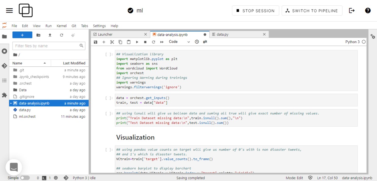
Running First Step
After debugging our code in Jupyter, it’s time to run our step by clicking on Switch to Pipeline. Select the Data step and run it. It takes a few seconds, and you can see on the sidebar the output of the step.
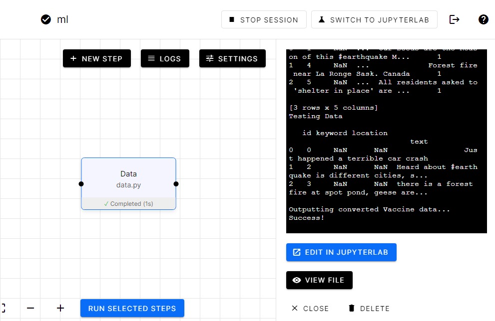
You can see in the image above how we will be using JupyterLab within Orchest Platform.
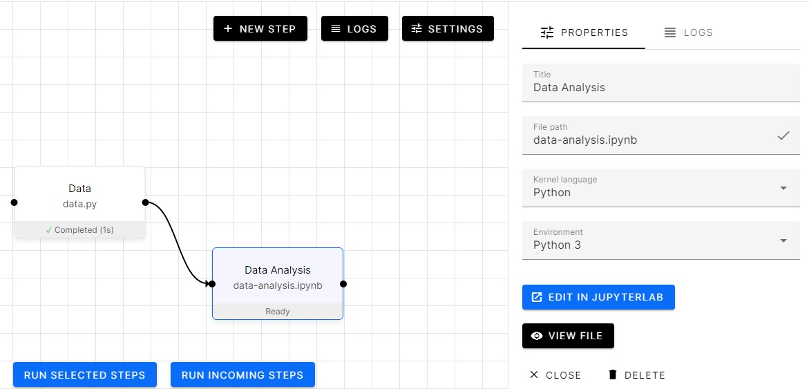
Adding data analysis step
Let’s add another step called “Data Analysis” we will be creating ipynb so that we can view each cell output in notebook format.
- Checking missing values
- Distribution of Target values
- Location distribution
- Word cloud for Disaster and Non-Disaster tweets
## Visualization library
import matplotlib.pyplot as plt
import seaborn as sns
from wordcloud import WordCloud
import orchest
## Ignoring Warning during trainings
import warnings
warnings.filterwarnings('ignore')
data = orchest.get_inputs()
train, test = data["data"]
## using isnull will give us bollean data and suming all true will give exact number of missing values.
print("Train Dataset missing data:n",train.isnull().sum(),"n")
print("Test Dataset missing data:n",test.isnull().sum())
Train Dataset missing data:
 id             0
keyword       61
location    2533
text           0
target         0
dtype: int64
Test Dataset missing data:
 id             0
keyword       26
location    1105
text           0
dtype: int64
VCtrain=train['target'].value_counts().to_frame()
## seaborn barplot to display barchart
sns.barplot(data=VCtrain,x=VCtrain.index,y="target",palette="viridis")
## Going deep into disaster Tweets
display("Random sample of disaster tweets:",train[train.target==1].text.sample(3).to_frame())
display("Random sample of non disaster tweets:",train[train.target==0].text.sample(3).to_frame())
'Random sample of disaster tweets:'
text
3606	Boy 11 charged with manslaughter in shooting d...
6055	Gaping sinkhole opens up in Brooklyn New York ...
5091	3 former executives to be prosecuted in Fukush...
'Random sample of non disaster tweets:'
text
5227	What a win by Kerry. 7-16..... #obliteration
3973	@crabbycale OH MY GOD THE MEMORIES ARE FLOODIN...
1017	@SlikRickDaRula Drake really body bagging peep...
#Locations
train.location.value_counts()[:10].to_frame()
| location | |
|---|---|
| USA | 104 |
| New York | 71 |
| United States | 50 |
| London | 45 |
| Canada | 29 |
| Nigeria | 28 |
| UK | 27 |
| Los Angeles, CA | 26 |
| India | 24 |
| Mumbai | 22 |
Word Cloud
disaster_tweets = train[train['target']==1]['text']
non_disaster_tweets = train[train['target']==0]['text']
fig, (ax1, ax2) = plt.subplots(1, 2, figsize=[16, 8])
wordcloud1 = WordCloud( background_color='white',
                        width=600,
                        height=400).generate(" ".join(disaster_tweets))
ax1.imshow(wordcloud1)
ax1.axis('off')
ax1.set_title('Disaster Tweets',fontsize=40);
wordcloud2 = WordCloud( background_color='white',
                        width=600,
                        height=400).generate(" ".join(non_disaster_tweets))
ax2.imshow(wordcloud2)
ax2.axis('off')
ax2.set_title('Non Disaster Tweets',fontsize=40);
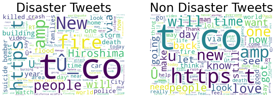
As you can see in the image below shows how we are going to use individual cells to perform data analysis.
Let’s run the Data Analysis step and as you can see in the image below that it’s taking the data from the “Data” step and using it to analyze both train and test data sets.
In this case, we are using -> data = orchest.get_inputs(); train, test = data[“data”]. The code is quite simple and easy to understand if you have been doing data visualization in past so I won’t be going deep into the coding part.

Preprocessing using Orchest
From now onward we are going to create steps and start adding code. We will be using the orchest library to transfer data from one step to another as mentioned before.
Let’s start by loading the data from the Data step.
## NLP library
import re
import string
import nltk
from nltk.corpus import stopwords
## ML Library
from sklearn.feature_extraction.text import CountVectorizer,TfidfVectorizer, TfidfTransformer
from sklearn.model_selection import RepeatedStratifiedKFold,cross_val_score
from sklearn.linear_model import LogisticRegression
from sklearn.naive_bayes import MultinomialNB
from sklearn.pipeline import Pipeline
from sklearn.metrics import f1_score
from sklearn.model_selection import train_test_split
import pickle
import orchest
RequestsDependencyWarning)
data = orchest.get_inputs()
train, test = data["data"]
train.text.head()
0 Our Deeds are the Reason of this #earthquake M...
1 Forest fire near La Ronge Sask. Canada
2 All residents asked to 'shelter in place' are ...
3 13,000 people receive #wildfires evacuation or...
4 Just got sent this photo from Ruby #Alaska as ...
Name: text, dtype: object
Text Cleaning
In this part, we are going to remove special characters, weblinks, and punctuations.
def text_processing(data):
# lowering the text
data.text=data.text.apply(lambda x:x.lower() )
#removing square brackets
data.text=data.text.apply(lambda x:re.sub('[.*?]', '', x) )
data.text=data.text.apply(lambda x:re.sub('+', '', x) )
#removing hyperlink
data.text=data.text.apply(lambda x:re.sub('https?://S+|www.S+', '', x) )
#removing puncuation
data.text=data.text.apply(lambda x:re.sub(
'[%s]' % re.escape(string.punctuation), '', x
))
data.text=data.text.apply(lambda x:re.sub('n' , '', x) )
#remove words containing numbers
data.text=data.text.apply(lambda x:re.sub('w*dw*' , '', x) )
return data
train = text_processing(train)
test = text_processing(test)
train.text.head()
0 our deeds are the reason of this earthquake ma...
1 forest fire near la ronge sask canada
2 all residents asked to shelter in place are be...
3 people receive wildfires evacuation orders in...
4 just got sent this photo from ruby alaska as s...
Name: text, dtype: object
Tokenization
token=nltk.tokenize.RegexpTokenizer(r'w+')
#applying token
train.text=train.text.apply(lambda x:token.tokenize(x))
test.text=test.text.apply(lambda x:token.tokenize(x))
#view
display(train.text.head())
0 [our, deeds, are, the, reason, of, this, earth...
1 [forest, fire, near, la, ronge, sask, canada]
2 [all, residents, asked, to, shelter, in, place...
3 [people, receive, wildfires, evacuation, order...
4 [just, got, sent, this, photo, from, ruby, ala...
Name: text, dtype: object
Removing stop words
Removing stop word improve the model performance in most cases.
nltk.download('stopwords')
#removing stop words
train.text=train.text.apply(lambda x:[w for w in x if w not in stopwords.words('english')])
test.text=test.text.apply(lambda x:[w for w in x if w not in stopwords.words('english')])
#view
train.text.head()
[nltk_data] Downloading package stopwords to /home/jovyan/nltk_data...
[nltk_data] Unzipping corpora/stopwords.zip.
0 [deeds, reason, earthquake, may, allah, forgiv...
1 [forest, fire, near, la, ronge, sask, canada]
2 [residents, asked, shelter, place, notified, o...
3 [people, receive, wildfires, evacuation, order...
4 [got, sent, photo, ruby, alaska, smoke, wildfi...
Name: text, dtype: object
Stemming
#stemmering the text and joining
stemmer = nltk.stem.PorterStemmer()
train.text=train.text.apply(lambda x:" ".join(stemmer.stem(token) for token in x))
test.text=test.text.apply(lambda x:" ".join(stemmer.stem(token) for token in x))
#View
train.text.head()
0 deed reason earthquak may allah forgiv us
1 forest fire near la rong sask canada
2 resid ask shelter place notifi offic evacu she...
3 peopl receiv wildfir evacu order california
4 got sent photo rubi alaska smoke wildfir pour ...
Name: text, dtype: object
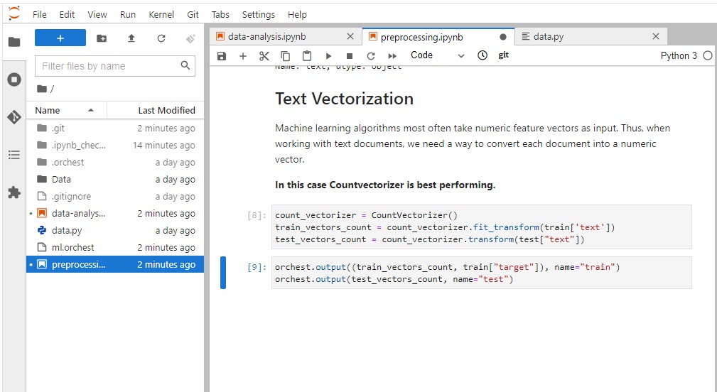
Text Vectorization
Machine learning algorithms most often take numeric feature vectors as input. Thus, when working with text documents, we need a way to convert each document into a numeric vector.
In our case, Countvectorizer is the best performing. We will be splitting your train dataset into train and validation.
vectorizer = TfidfVectorizer()
train_vectors_count = vectorizer.fit_transform(train['text'])
test_vectors_count = vectorizer.transform(test["text"])
X_train, X_val, y_train, y_val = train_test_split(train_vectors_count, train["target"], test_size=0.2, random_state=40,stratify=train["target"])
orchest.output((X_train, y_train,X_val, y_val,test_vectors_count), name='train_val_test')
As we can see in the image below how I used Jupyter notebook to run experiments and come up with a better solution. Once you have built a pipeline you can make changes and evaluate your model’s performance easily.
EvalML: AutoML
We will be using EvalML for our AutoML step so that we can pick which models performed better. The code below is quite simple and easy to understand and if you want to know more about various ways you can train your model you can check out EvalML 0.35.0 documentation
EvalML is an AutoML library that builds, optimizes, and evaluates machine learning pipelines using domain-specific objective functions.
Key Functionality
- Automation – Makes machine learning easier. Avoid training and tuning models by hand. Includes data quality checks, cross-validation, and more.
- Data Checks – Catches and warns of problems with your data and problem setup before modeling.
- End-to-end – Constructs and optimizes pipelines that include state-of-the-art preprocessing, feature engineering, feature selection, and a variety of modeling techniques.
- Model Understanding – Provides tools to understand and introspect on models, to learn how they’ll behave in your problem domain.
- Domain-specific – Includes repository of domain-specific objective functions and an interface to define your own.
import orchest ## EVALML from evalml.automl import AutoMLSearch from sklearn.model_selection import train_test_split from sklearn.metrics import f1_score import warnings warnings.filterwarnings("ignore")/opt/conda/lib/python3.7/site-packages/requests/__init__.py:91: RequestsDependencyWarning: urllib3 (1.26.7) or chardet (3.0.4) doesn't match a supported version! RequestsDependencyWarning)
data = orchest.get_inputs() train,test = data["data"]X = train.drop(['target'], axis=1) y = train['target']import woodwork as ww # X = ww.DataTable(X) # Note: We could have also manually set the text column to # natural language if Woodwork had not automatically detected from evalml.utils import infer_feature_types X = infer_feature_types(X, {'text': 'NaturalLanguage'}) # y = ww.DataColumn(y)from evalml.preprocessing import split_data X_train, X_holdout, y_train, y_holdout = split_data(X, y, problem_type='binary', test_size=0.2)automl = AutoMLSearch(X_train=X_train, y_train=y_train,additional_objectives=['f1'], problem_type='binary',max_time=300)automl.search()%%time pipeline = automl.best_pipeline pipeline.fit(X_train, y_train)CPU times: user 7.44 s, sys: 437 ms, total: 7.88 s Wall time: 7.28 s
pipeline = BinaryClassificationPipeline(component_graph={'Drop Columns Transformer': ['Drop Columns Transformer', 'X', 'y'], 'Text Featurization Component': ['Text Featurization Component', 'Drop Columns Transformer.x', 'y'], 'Imputer': ['Imputer', 'Text Featurization Component.x', 'y'], 'One Hot Encoder': ['One Hot Encoder', 'Imputer.x', 'y'], 'XGBoost Classifier': ['XGBoost Classifier', 'One Hot Encoder.x', 'y']}, parameters={'Drop Columns Transformer':{'columns': ['location']}, 'Imputer':{'categorical_impute_strategy': 'most_frequent', 'numeric_impute_strategy': 'mean', 'categorical_fill_value': None, 'numeric_fill_value': None}, 'One Hot Encoder':{'top_n': 10, 'features_to_encode': None, 'categories': None, 'drop': 'if_binary', 'handle_unknown': 'ignore', 'handle_missing': 'error'}, 'XGBoost Classifier':{'eta': 0.1, 'max_depth': 6, 'min_child_weight': 1, 'n_estimators': 100, 'n_jobs': -1, 'eval_metric': 'logloss'}}, random_seed=0)
preds = pipeline.predict(X_holdout)print("F1 score:",f1_score(y_holdout,preds)) orchest.output(automl,name='automl')F1 score: 0.6962457337883959
Results
Let’s create another step for the AutoML step which displays the best performing libraries.
import orchestdata = orchest.get_inputs() automl = data["automl"]automl.rankingsorchest.output(automl.rankings,name='automl_results')best_pipeline_id = automl.rankings.iloc[0]["id"] automl.describe_pipeline(best_pipeline_id)************************************************************************************************************* * XGBoost Classifier w/ Drop Columns Transformer + Text Featurization Component + Imputer + One Hot Encoder * ************************************************************************************************************* Problem Type: binary Model Family: XGBoost Pipeline Steps ============== 1. Drop Columns Transformer * columns : ['location'] 2. Text Featurization Component 3. Imputer * categorical_impute_strategy : most_frequent * numeric_impute_strategy : mean * categorical_fill_value : None * numeric_fill_value : None 4. One Hot Encoder * top_n : 10 * features_to_encode : None * categories : None * drop : if_binary * handle_unknown : ignore * handle_missing : error 5. XGBoost Classifier * eta : 0.1 * max_depth : 6 * min_child_weight : 1 * n_estimators : 100 * n_jobs : -1 * eval_metric : logloss Training ======== Training for binary problems. Total training time (including CV): 46.9 seconds Cross Validation ---------------- Log Loss Binary F1 # Training # Validation 0 0.531 0.675 4,060 2,030 1 0.582 0.657 4,060 2,030 2 0.556 0.678 4,060 2,030 mean 0.556 0.670 - - std 0.026 0.011 - - coef of var 0.046 0.017 - -
automl.best_pipeline.component_graph.graph()Drop Columns Transformer columns : ['location'] Text Featurization Component Imputer categorical_impute_strategy : most_frequent numeric_impute_strategy : mean categorical_fill_value : None numeric_fill_value : None One Hot Encoder top_n : 10 features_to_encode : None categories : None drop : if_binary handle_unknown : ignore handle_missing : error XGBoost Classifier eta : 0.10 max_depth : 6 min_child_weight : 1 n_estimators : 100 n_jobs : -1 eval_metric : logloss X y
Logistic Regression-
We are going to create three more steps that will take data from pre-processed step and run various classification models.
- Building LogisticRegression with default hyperparameters.
- Running Repeated Stratified K-fold
- Observing scores for every fold
- Finally, train and evaluate our model
Not bad 0.75 F1 scores is quite good for the vanilla model.
We will be using this code and changing the model’s name for the other three steps.
- Naive Bayes
- Light GBM
- Random Forest
import orchest
from sklearn.metrics import f1_score
import warnings
warnings.filterwarnings("ignore")
from sklearn.model_selection import RepeatedStratifiedKFold,cross_val_score
from sklearn.linear_model import LogisticRegression

data = orchest.get_inputs()
X_train,y_train, X_val,y_val,test = data["train_val_test"]
LR = LogisticRegression()
cv = RepeatedStratifiedKFold(n_splits=5, n_repeats=3, random_state=1)
scores = cross_val_score(LR, X_train, y_train, cv=cv, scoring="f1")
scores
array([0.70939227, 0.7405765 , 0.74273412, 0.69690265, 0.73456121,
       0.72246696, 0.70509978, 0.68673356, 0.75349839, 0.70792617,
       0.70707071, 0.72668113, 0.7211329 , 0.72766885, 0.72628135])
LR.fit(X_train,y_train)
y_pred = LR.predict(X_val)
print("F1 score :", f1_score(y_pred, y_val))
F1 score : 0.7532244196044712
orchest.output((LR, y_pred,),name="LR")
Ensemble-
We are going to create an Ensemble step that will take the data from all three models step and use VotingClassifier to train and evaluate the results.
- Ingesting all four-model data
- Building Voting Classifier model using all four models
- Train model on train dataset
- Evaluating model on the validation dataset
- Evaluating by displaying confusing matrix in form of a heatmap.
We got a 0.73 F1 score which is worse than simple logistic regression.
import orchest
import seaborn as sns
import matplotlib.pyplot as plt
from sklearn.ensemble import RandomForestClassifier,VotingClassifier
from sklearn.metrics import f1_score,accuracy_score,classification_report,confusion_matrix
/opt/conda/lib/python3.7/site-packages/requests/__init__.py:91: RequestsDependencyWarning: urllib3 (1.26.7) or chardet (3.0.4) doesn't match a supported version!
  RequestsDependencyWarning)
data = orchest.get_inputs()
lgbm, pred_lgbm = data["lgbm"]
rf, pred_rf, X_train, y_train, X_val, y_val, test = data["RF"]
nb, pred_nb = data["NB"]
lr, pred_lr = data["LR"]
total_score=[]
model = VotingClassifier(
    estimators=[("lr", lr), ("RF", rf), ("NB", nb), ("LGBM", lgbm)],
    voting="hard",
)
model.fit(X_train, y_train)
# Make predictions
y_pred = model.predict(X_val)
f1_score = f1_score(y_val, y_pred)
# Check the F1 score of the model
print("F1 score:", f1_score)
F1 score: 0.7347670250896057
accuracy_score = accuracy_score(y_val,y_pred)
print("Accuracy Score:",accuracy_score)
Accuracy Score: 0.8056467498358503
plt.figure(figsize=(10, 10))
cm = confusion_matrix(y_val, y_pred)
sns.heatmap(
    cm,
    cmap="Blues",
    linecolor="black",
    linewidth=1,
    annot=True,
    fmt="",
    xticklabels=["Covid_Negative", "Covid_Positive"],
    yticklabels=["Covid_Negative", "Covid_Positive"],
)
plt.xlabel("Predicted")
plt.ylabel("Actual")
.png)
orchest.output((model, test, f1_score, accuracy_score),name='ensemble')
I have skipped few steps as they were following similar patterns. If you want to see the entire pipeline with the code, you should check out my GitHub repository. kingabzpro/ML-Pipeline-Disaster-tweets
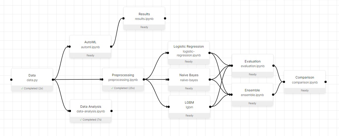
Final Pipeline using Orchest
Our final pipeline contains:
- Data: Data ingestion from CVS files.
- Data Analysis: Visualization and Analyzing tweets distributions
- Preprocessing: Cleaning, tokenization stammering, and splitting the dataset
- Automl: Using EvalML to train with few lines of code
- Results: Analyzing AutoML results
- Logistic Regression: Training simple Logistics classifier
- Naïve Bayes: Training and evaluation
- LGBM: Training and evaluating
- Random Forest: Training and evaluating
- Evaluation: Evaluating all the models
- Ensemble: ensembling all three models
- Comparison: comparing ensemble model results with simple models
- Submission: predicting the test dataset and preparing submission files.
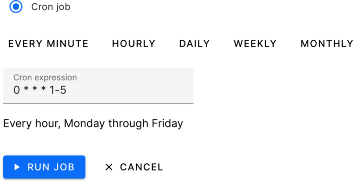
Schedule executions using Orchest
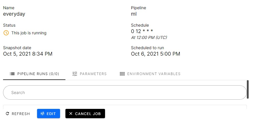
We are creating the job by clicking on the jobs tab to schedule run this pipeline every 24 hours.
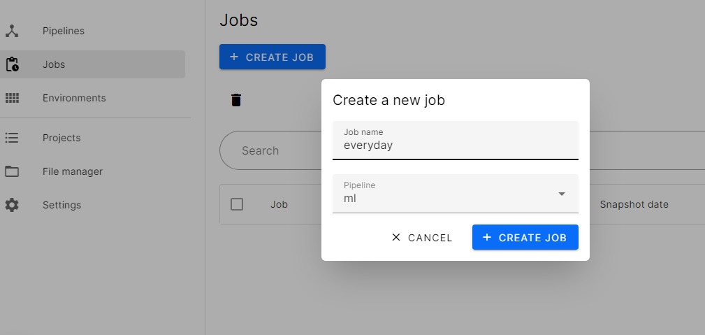
As you can see in the image below of our job in the process. It will run at 12 pm UTC every day until we cancel the job. You can also add parameters and environment variables if you are using an external dataset or API.
Results
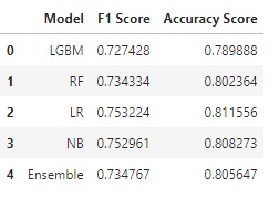
The results are here from the comparison step and logistic regression performed best among all, whereas Light GBM performed worst. We will be using this result to select a single model and predict targets for test datasets.
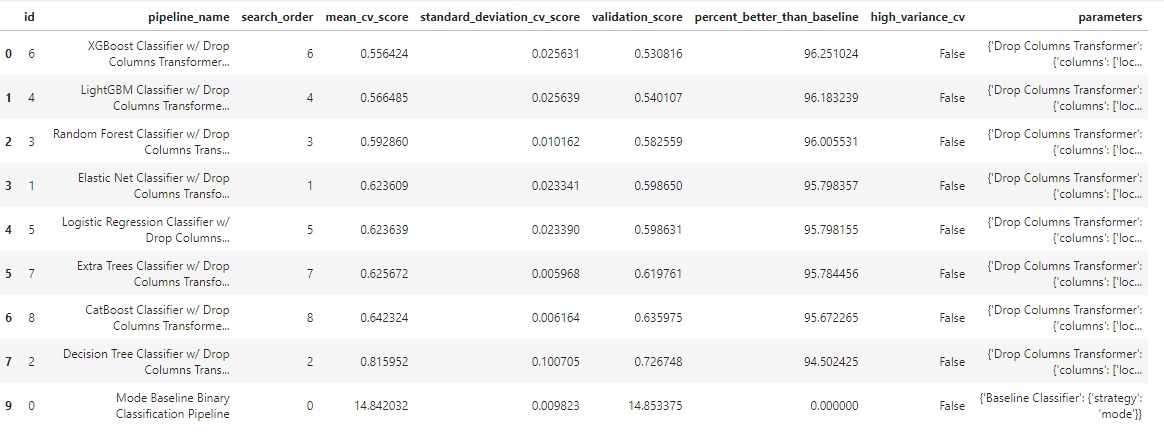
AutoML Results
The AutoML results are worse than any model that I have mentioned above. Maybe If we had them through preprocessed data the results would be better.
You can see in the image below the pipelines and the results.
Submission
In the submission step, the best-performing model and test dataset are ingested. We will be also loading the sample_submission file using pandas read_csv.
- Predicting on the test dataset
- Adding prediction to target
- Exploring submission files in CSV format
- Submitting to Kaggle competition Natural Language Processing with Disaster Tweets | Kaggle
import pandas as pd
import orchest
  RequestsDependencyWarning)
sub = pd.read_csv("Data/sample_submission.csv")
data = orchest.get_inputs()
model,test = data["sub"]
pred_test = model.predict(test)
sub["target"] = pred_test
sub.head()
id	target
0	0	0
1	2	1
2	3	1
3	9	1
4	11	1
sub.to_csv("submission.csv",index=False)
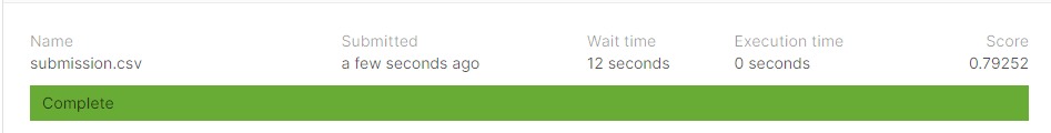
As you can our model performed quite well on a private dataset with 0.792 F1 scores.
Conclusion
In this guide, we have learned how we can divide our machine learning parts into different steps and how every step is using dataflow to process the data and exporting it for the next step. We have also learned to create various steps in the pipeline and use Jupyter notebook to code the machine learning data flow.
In my opinion, the world is shifting towards machine learning pipelines as they provide flexibility and scalability. You can also add Weights & Biases for experiment tracking or other integrations such as using Streamlit to create a web app.
There is more to just creating a data pipeline in Orchest. The platform provides you with all the tools that data scientists are familiar with. I love every bit as I was creating this guide and experimented with various features. Finally, after evaluating and creating the submission file we have successfully achieved almost the best score on a private dataset. Next time we will be learning more exciting MLOps tools to make your life easy. The MLOPs is the future of AI and if you want to increase your odds of getting hired by top companies in your country, start investing in MLOPs tools.
Code
You can find the entire project on GitHub and DAGsHub
Learning Resources
- Data analysis on competition data feature engineering ideas for NLP, cleaning, and text processing ideas, baseline BERT model or test set with labels: NLP with Disaster Tweets – EDA, Cleaning and BERT | Kaggle
- Step by step guide to perform tweet analysis: Tweet analytics using NLP
- Natural Language Processing and Tweet Sentiment Analysis: Medium Article by Cassandra Corrales
- Designing your first machine learning pipeline with a few lines of codes using Orchest: A New Way of Building Machine Learning Pipelines
Orchest Sample Projects
- Designing your first machine learning pipeline with few lines of codes using Orchest. You will learn to preprocess the data, train the machine learning model, and evaluate the results: kingabzpro/Covid19-Vaccine-ML-Pipeline
- This repository demonstrates an Orchest pipeline that generates an audio fragment using the Quoki TTS engine and sends it as a message on Slack: ricklamers/orchest-coqui-tts
About Author
Abid Ali Awan (@1abidaliawan) is a certified data scientist professional who loves building machine learning models and research on the latest AI technologies. Currently testing AI Products at PEC-PITC, their work later gets approved for human trials, such as the Breast Cancer Classifier.
Image Source:
- Image 1 – https://www.freepik.com/free-vector/pipeline-maintenance-concept-illustration_13795579.htm#page=1&query=pipeline&position=45&from_view=search
- Image 2 – https://docs.microsoft.com/en-us/azure/machine-learning/service/concept-ml-pipelines
- Image 3 – https://www.algorithmia.com/blog/ml-pipeline
- Image 4 – https://www.orchest.io/?ref=producthunt
I am a technology manager turned data scientist who loves building machine learning models and research on various AI technologies. My vision is to build an AI product that will help identify students who are struggling with mental illness.


