Classifying Sexual Harassment Personal Stories!

Introduction

We can make use of Machine Learning in order to categorize such harassment incidents without any manual human intervention. Traditionally if a report needs to file regarding a harassment case, the victim needs to provide the description of the case along with filling up several forms. We can automate some parts of this process by categorizing the incidents based on the descriptions and then performing further processes based on the category of the cases. This automatic classification of different forms of sexual harassment will immensely help the authorities as well as the concerned organizations to partially automate their systems that file reports against such incidents.

How do we pose this as ML Problem?

Here our objective is to use short stories which were submitted online and to be able to automatically categorize each story submitted by a user. We will consider the user stories as our training data. We will try to build a Machine Learning model which will take these stories/descriptions as input and try to predict the categories of harassment it belongs to. The main thing to keep in mind here is that a description may belong to multiple categories. For example, a description could indicate both Commenting and Groping cases.

Data-Source : https://github.com/swkarlekar/safecity
Authors: Sweta Karlekar & Mohit Bansal, University of North Carolina at Chapel Hill

The dataset has 7201 training samples, 990 validation samples, and 1701 test samples. Each data sample consists of a Description of the incident followed by whether it belongs to classes Commenting, Staring, and Groping. As it is a Multi-Label classification problem, each data point can belong to multiple classes.

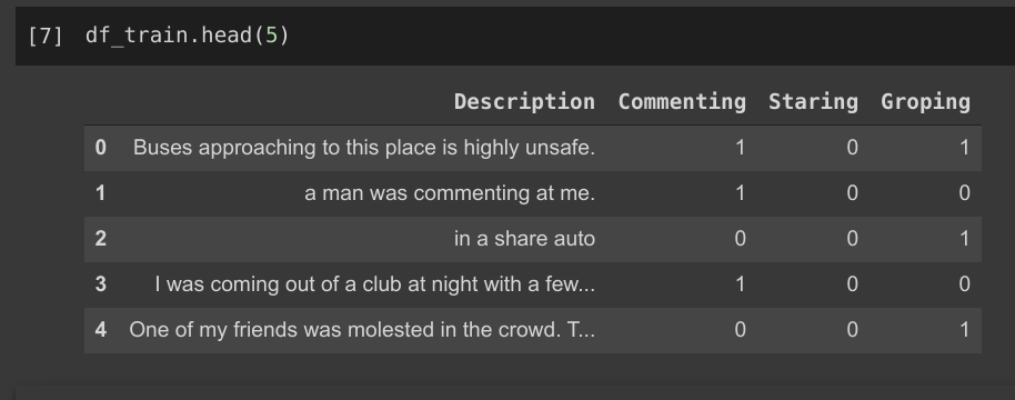
Dataset Example

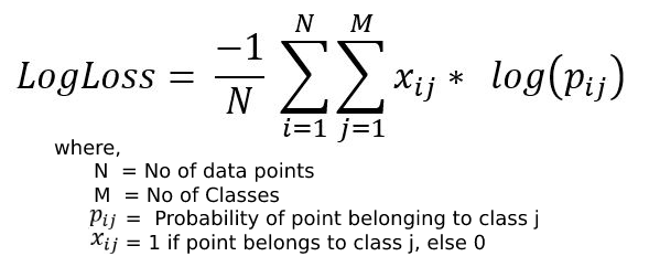
Performance Metrics

Initially, this problem is a Multi-Label Classification problem, but later we will map it to a Multi-Class classification problem, hence we can use multi-class classification metrics for evaluating our model. We use the following metrics :

LogLoss: It is calculated as the average of negative log probabilities of the data point belonging to the correct class label. Log loss can range from 0 to infinity, lower LogLoss indicates that more points are classified correctly. In our case, LogLoss seems to be very helpful as we have multiple classes.

Precision: It gives us an idea about out of all the points predicted to belong to a certain class, how many actually do belong to that class.
Recall: Recall indicates out of all points belonging to a class, how many were actually correctly classified
F1-Score: It’s the Harmonic mean of Precision & Recall which tries to have higher values for both precision and recall. It ranges from 0(worst) to 1(best)

Exploratory Data Analysis

First, let’s have a look at the words of each description and how they can help us to gain insights into the classification. We find the top 15 most frequent words for each category and plot them.

No of Labels

We count the no_of_labels each data point belongs to. This leads to the following observations :

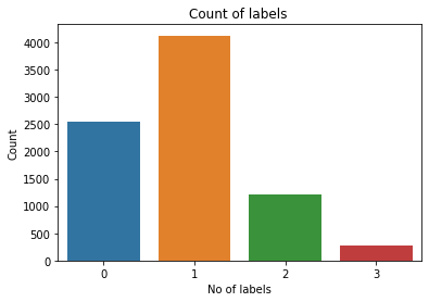
• 2557 (31%) data points do not belong to any classes
• 4128 (50%) data points belong to only 1 class which is significantly higher than others
• Only 19.4% of points have multiple labels i.e belong to multiple classes ( >1 label)

Venn Diagram

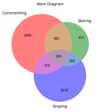
• 31% of data points don’t belong to any class & 284 (3%) Data points belong to all 3 classes
• There is significantly lesser overlap between Groping and Staring while there is a larger overlap between Commenting and staring

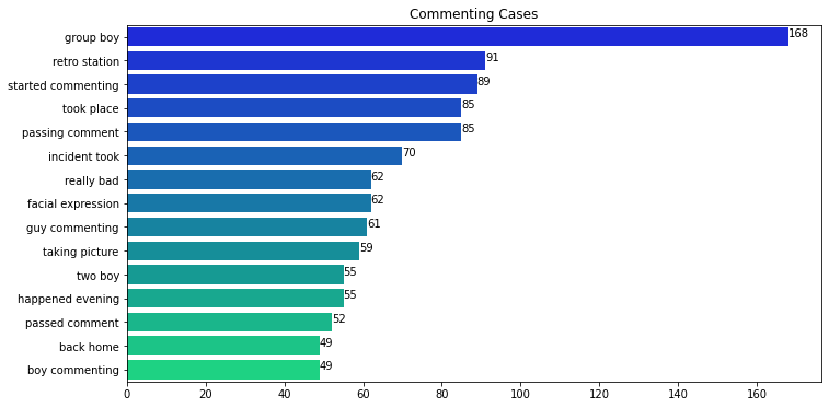
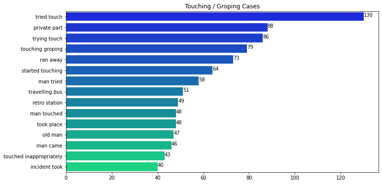
Frequent Words

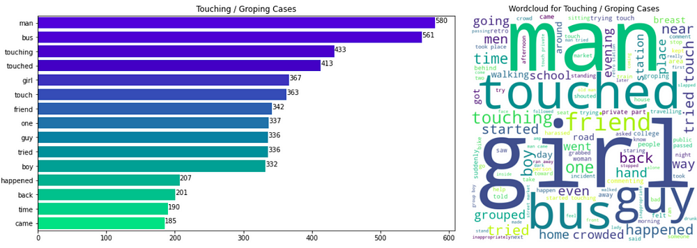
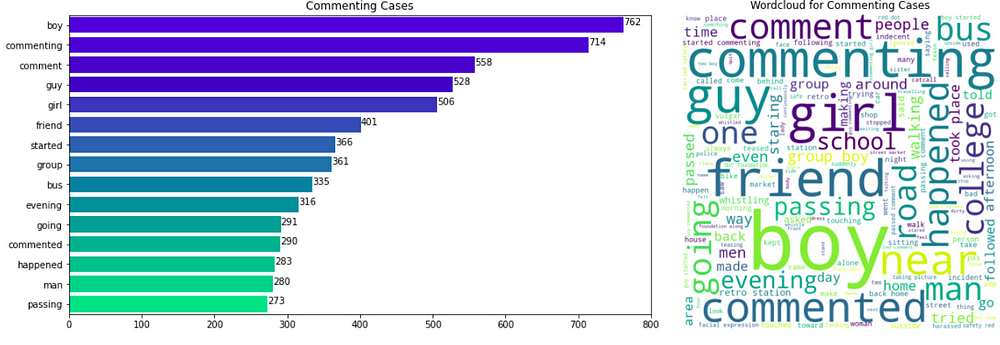
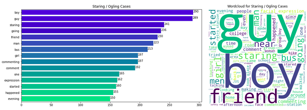
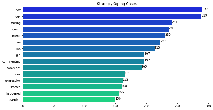
We find the top 15 most frequent words in each class label case and plot the frequency of these words. Also, for visual representation, we also plot the word cloud using the text corpus for each label.

Observations

• Groping Cases: The words ‘man’, ‘bus’, ‘touching’, and ‘touched’ are the most frequent 4 words. The words like ‘bus’ make perfect sense as most groping cases may happen in crowded places like buses.
• Commenting Cases: Words ‘boy’ and ‘commenting’ occur 762,714 times which is almost 30–40% more than the next frequent word i.e comment, guy, etc
• We can see that some words appear commonly in all 3 classes: 7 words (‘man’, ‘bus’, ‘happened’, ‘friend’, ‘girl’, ‘guy’, ‘boy’) appear in the top-10 most frequent words in all 3 classes. Hence, we can conclude that these insights cannot help our decision process much as they appear in all 3 classes

Similarly, we can also have a look at the most frequent bigrams (2-words)

Length of Descriptions

We count the no of words in each description and plot the Distributions as well as percentile values.

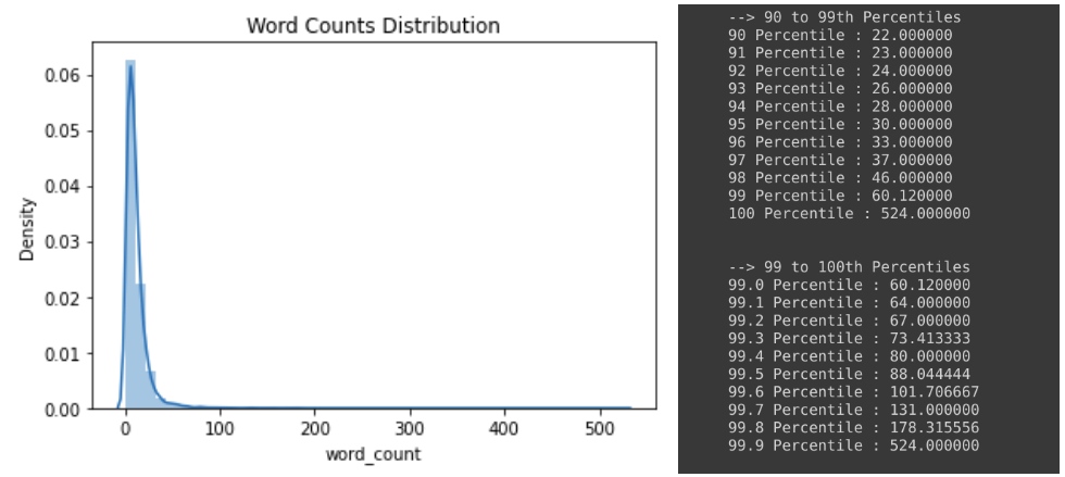
• From the Word Counts Distribution, we found that only 29+5 = 34 samples had word_counts > 100
• When we look at the percentiles, we find that 99% of the samples have word_count < 60 which indicated that the descriptions given by users are usually short and don’t include lengthy descriptions of the incident
• From the observations, we will consider word_count greater than 88(99.5th Percentile) as outliers.

Average Word Length

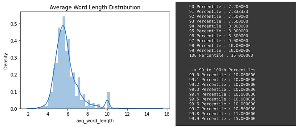
• Very few samples have average word length > 10 which is expected as most commonly used words in English are shorter than 10 characters
• 99% of the descriptions had average word length <= 10 and around 90% had average <= 8.
• From the above observation, we will consider samples having average word length > 10(99.7th percentiles) as outliers.

Data Visualization

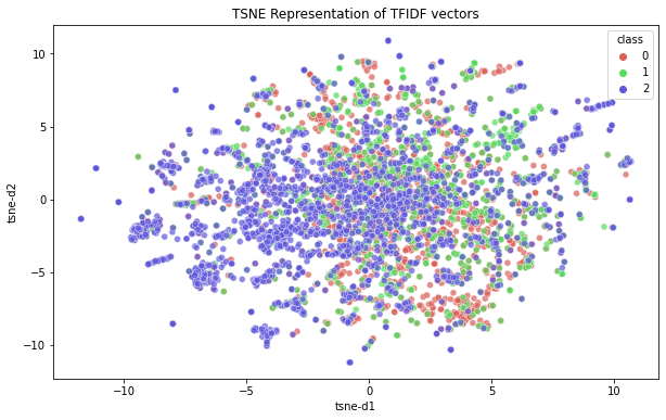
We first used TF-IDF vectorizer to convert word data into a numerical representation.
1. We first use PCA to reduce the dimensions to 100
2. We then use t-SNE to reduce and visualize the data in 2 dimensions
As we can from the plot below, we cannot distinguish the classes using 2d t-SNE representations.

Data Preprocessing

We follow the following Sequence to clean the data

1. Decontract Words
2. Remove Special Symbols
3. Remove Stopwords
4. Remove HTML tags
5. Remove Punctuations
6. Lemmatize the sentence using WordNetLemmatizer

def pre_process_text(phrase):
    '''Clean and lemmatize text'''
    phrase = re.sub(r"won't", "will not", phrase)
    phrase = re.sub(r"can't", "can not", phrase)
    phrase = re.sub(r"n't", " not", phrase)
    phrase = re.sub(r"'re", " are", phrase)
    phrase = re.sub(r"'s", " is", phrase)
    phrase = re.sub(r"'d", " would", phrase)
    phrase = re.sub(r"'ll", " will", phrase)
    phrase = re.sub(r"'t", " not", phrase)
    phrase = re.sub(r"'ve", " have", phrase)
    phrase = re.sub(r"'m", " am", phrase)
    phrase = re.sub('[^A-Za-z0-9]+', ' ', phrase)
    phrase = ' '.join(e.lower() for e in phrase.split() if e.lower() not in stopwords.words('english'))
    cleanr = re.compile('')
    phrase = re.sub(cleanr, ' ', str(phrase))
    phrase = re.sub(r'[?|!|'|"|#]',r'',phrase)
    phrase = re.sub(r'[.|,|)|(||/]',r' ',phrase)
    phrase = phrase.strip()
    phrase = phrase.replace("n"," ")
    phrase = TextBlob(phrase).correct()
    lemmatizer = WordNetLemmatizer()
    lemmatized_sentence = " ".join([lemmatizer.lemmatize(word) for word in phrase.split(" ")])
    return str(lemmatized_sentence)

Feature Engineering

We try to extract features from the text descriptions which can help us further in classification. These are the features extracted

1. Length of Descriptions & Average Word Length

# Fing Average Length
df_train["avg_word_length"] = df_train["Description"].apply(lambda x: np.mean([len(word) for word in x.split(" ")]))
# Count Total Words
df_train["word_count"] = df_train["Description"].apply(lambda x: len(x.split(" ")))

2. Text Scoring Metrics

• Difficulty Score: It is a measure of the relative level of difficulty of the words used in the sentence
• flesch_reading_ease: It indicates how easy a text is to understand. The higher the score, the easier it is to understand the text
• flesch_kincaid_grade: It is based on the flesch_reading_ease which gives a score to text to judge the readability level of the text.

• coleman_liau_index: Intended to gauge the understandability of a text. It is similar to Flesch Score but relies on characters instead of syllables per word

To calculate these Text Scoring metrics we use the Textstat python library which provides functions to calculate the scores.

import textstat

df["word_count"] = df["Description"].apply(lambda x: len(x.split(" ")))
df["avg_word_length"] = df["Description"].apply(lambda x: np.mean([len(word) for word in x.split(" ")]))
df["difficult_words_score"] = df["Description"].apply(lambda x: textstat.difficult_words(x))
df["flesch_reading_ease"] = df["Description"].apply(lambda x: textstat.flesch_reading_ease(x))
df["flesch_kincaid_grade"] = df["Description"].apply(lambda x: textstat.flesch_kincaid_grade(x))
df["coleman_liau_index"] = df["Description"].apply(lambda x: textstat.coleman_liau_index(x))

3. Part of Speech Tagging

We can use the count_POS function used below to count the no of nouns, adverbs, verbs, adjectives, and pronouns in a given text.

pos_re = {"noun":re.compile('N.*'), "verb":re.compile('V.*'),
          "adverb":re.compile('R.*'), "adjective":re.compile('J.*'),
          "pronoun":re.compile('J.*')}
def count_POS(text, part_of_speech):
  count = 0
  for word, pos in nltk.pos_tag(word_tokenize(text)):
    if re.match(pos_re[part_of_speech],pos):
      count += 1
  return count
df["noun_count"] = df["Description"].apply(lambda x: count_POS(x,"noun"))
df["pronoun_count"] = df["Description"].apply(lambda x: count_POS(x,"pronoun"))
df["verb_count"] = df["Description"].apply(lambda x: count_POS(x,"verb"))
df["adverb_count"] = df["Description"].apply(lambda x: count_POS(x,"adverb"))
df["adjective_count"] = df["Description"].apply(lambda x: count_POS(x,"adjective"))

TF-IDF Weighted GloVe Embeddings

In order to convert our text descriptions into numerical representations, we use the TF-IDF Weighted GloVe Embeddings techniques using the following steps

• First, we load the pre-trained Glove vector and store the vector embeddings in a dictionary. The glove vector we use provides a 300-dimensional embedding vector for each word.
• For each sentence, we do a weighted TF-IDF sum. We first initialize a vector with 300 zeros. Then for each valid word in the sentence, we add glove_embedding[word] + tf_idf_score[word] to the vector and finally divide it by summation of tf_idf values.

# Load Glove Vector
with open('/content/glove.pickle', 'rb') as f:
  glove_vectors = pickle.load(f)
  glove_words = set(glove_vectors.keys())
# Calculate tf-idf values
tfidf_vec = TfidfVectorizer()
tfidf_vec.fit(df_train["Description"].values)
tfidf_dict = dict(zip(tfidf_vec.get_feature_names(), list(tfidf_vec.idf_)))
tfidf_words = set(tfidf_vec.get_feature_names())
# TF-IDF weighted W2V
def tfdidf_w2v(data, tf_idf_words, tfidf_dict):
  tfidf_w2v_vectors = []; 
  for sentence in data:
      vector = np.zeros(300) 
      tf_idf_weight =0
      for word in sentence.split(): 
          if (word in glove_words) and (word in tf_idf_words):
              vec = glove_vectors[word] 
              tf_idf = tfidf_dict[word]*(sentence.count(word)/len(sentence.split()))
              vector += (vec * tf_idf) 
              tf_idf_weight += tf_idf
      if tf_idf_weight != 0:
          vector /= tf_idf_weight
      tfidf_w2v_vectors.append(vector)
  return tfidf_w2v_vectors
train_data_embeddings = tfdidf_w2v(df_train["Description"].values)
test_data_embeddings = tfdidf_w2v(df_test["Description"].values)

Mapping from Multi-Label to Multi-Class Problem

To make it easier for us during modelling, as we have only 3 classes we try to pose this as a multi-class problem. A data point can belong to any of the 3 classes, hence we have 2³ = 8 classes. Thus we convert the problem into a multi-class classification problem with 8 classes. We then convert our Dataset labels according to these new classes.

Class 0: None (No Harassment)
Class 1: Staring
Class 2: Groping
Class 3: Commenting
Class 4: Commenting & Staring
Class 5: Staring & Groping
Class 6: Commenting & Groping
Class 7: Staring,Commenting & Groping

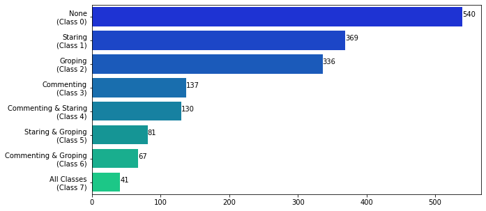
We can notice that majority of the data belongs to Class 0. Classes 0,1 and 2 also have a relatively higher number of samples. This imbalance needs to be taken into consideration while we evaluate our predictions after modeling.

At the end of Feature engineering, we stack all the newly created features together. For each data point, we have 311 features and we get Train Data shape: (8189, 311) and Test Data Shape: (1701, 311)

311 Features = TF-IDF Weighted GloVe Embeddings (300) + Word_Count + Average_Word_Count + Difficulty Score + flesch_reading_ease + coleman_liau_index +flesch_kincaid_grade +noun_count + pronoun_count +verb_count + adjective_count +adverb_count

ML Model Building

For plotting the evaluation metrics we use we will define a function plot_metrics(). It will take the trained model as an argument and print all the needed metrics.

LogLoss = make_scorer(log_loss, greater_is_better=False, needs_proba=True)

def plot_confusion_matrix(test_y, predict_y):
  skplt.metrics.plot_confusion_matrix(test_y, predict_y,normalize=True,figsize=(13,7),cmap='Blues')
  plt.show()

def print_metrics(built_model):
  print("*-*-*-**-*-*-TRAIN METRICS*-*-*-*-*-*-")
  logLoss = log_loss(y_train, built_model.predict_proba(X_train))
  f1Score = f1_score(y_train, built_model.predict(X_train), average='weighted')
  print("Log Loss: ", logLoss)
  print("Precision : ",precision_score(y_train,built_model.predict(X_train),average='weighted'))
  print("Recall : ",recall_score(y_train,built_model.predict(X_train),average='weighted'))
  print("F1-Score : ",f1Score)
  print("n*-*-*-**-*-*-TEST METRICS*-*-*-*-*-*-")
  logLoss = log_loss(y_test, built_model.predict_proba(X_test))
  f1Score = f1_score(y_test, built_model.predict(X_test), average='weighted')
  print("Log Loss: ", logLoss)
  print("Precision : ",precision_score(y_test,built_model.predict(X_test),average='weighted'))
  print("Recall : ",recall_score(y_test,built_model.predict(X_test),average='weighted'))
  print("F1-Score : ",f1Score)
  plot_confusion_matrix(y_test, built_model.predict(X_test))

Dummy Classifier

As the initial step, we will build a Dummy Classifier which acts as a benchmark for evaluating other models. We use the DummyClassifier model provided by sklearn which randomly classifies data.

We get a Log Loss of 26.80 for the test dataset. This value can be used as a baseline, if any model gives us a loss greater than this, then we can say that its performance is even worse compared to a random model.

Logistic Regression
We train a Logistic Regression model with the dataset. Hyperparameter tuning is done using RandomizedSearchCV which gives us the best model with the optimal parameters.

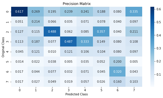
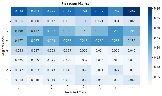
From the results, we can see that on test data our Logistic Regression model performs a lot better than our Dummy Classifier. But, looking at the Precision Matrix we can see that the model favors the majority classes. A higher number of samples belonging to the majority classes were predicted correctly. Very few points were predicted to belong to classes 5, 6, and 7 which are the minority classes.

XGBoost

params = {'max_depth':randint(1,50),"n_estimators":randint(10,200)}
xgb_hyp = RandomizedSearchCV(
  					XGBClassifier(),
  					param_distributions=params, 		
  					verbose=1,n_jobs=-1,
  					scoring=LogLoss)
xgb_hyp.fit(X_train,y_train)
print_metrics(xgb_hyp)

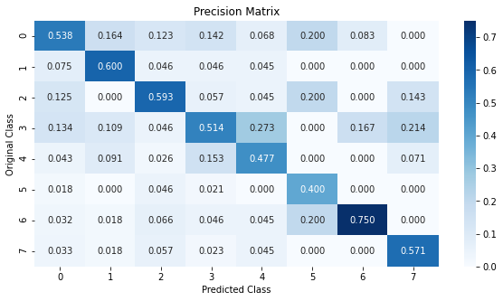
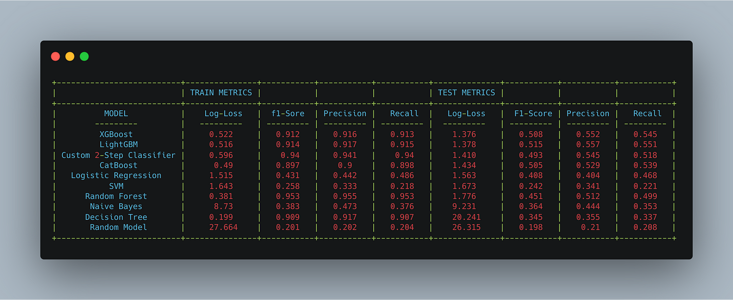
We observe that using XGBoost the test LogLoss reduced to 1.3763 from 1.5633 when compared to the Logistic Regression model. Also, the precision matrix indicates that we predict the classes better and majority classes are not favored too much. Even classes 5, 6, 7 are better predicted when compared to Logistic Regression Model.

Exploring other models
We tried using other ML models to check if we can reduce the loss further. For each algorithm, we performed hyperparameter tuning to get the best parameters. The models we experimented with are: XGBoost
LightGBM, CatBoost, Logistic Regression, SVM, Random Forest,
Naive Bayes and Decision Tree.

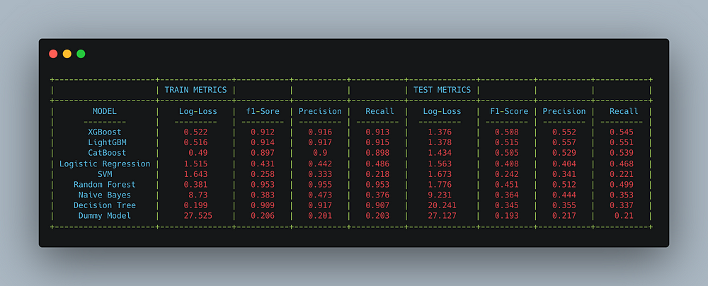
Ensemble models like XGBoost, LightGBM & CatBoost performed Significantly better when compared to other algorithms

Custom 2-Step Classifier

As we noticed the majority of the classes belong to class 0, due to this when we observe the Confusion matrix of the trained models we see that the predictions favor Class 0. So in order to fix this issue, we try to build a model which follows a 2-step classification approach.

• Model 1: Classify if the data belongs to class = 0 or not.
  For training this model we modify the dataset as follows: if class ≥ 1, the label=0 else label = 1
• Model 2: If model 1 predicts class != 0, then predict the label from class 1–7. For training this model we only use points in the dataset which belong to Class 1–7

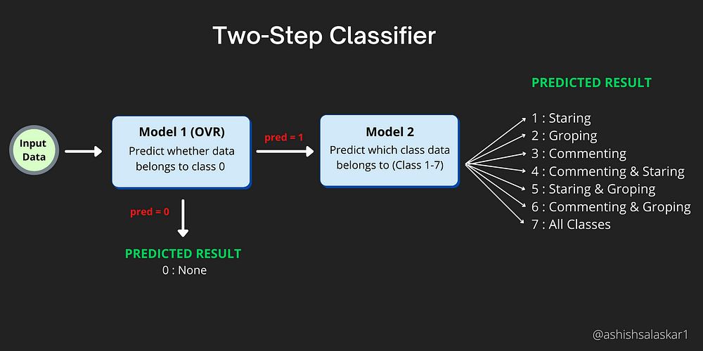
Prediction Steps: Here we first pass the data to be predicted to Model 1 first, it checks if the sample belongs to Class 0 or not. If it doesn’t belong to class 0 then we pass the sample to Model 2 which can then predict if the sample belongs to Classes 1 to 7.

We implement this models as a TwoStepClassifier class. It has these methods
1. load_models(model1, model2) : We need to pass the trained model1 & model 2 to this function.
2. predict_proba() and predict() are used for prediction
3. get_metrics() : prints the metrics

Comparing all the models

When we compare the overall models, XGBoost and LightGBM perform significantly better than other algorithms. Our custom 2-Step-Classifier also performed better than most algorithms but not as good as XGBoost & LightGBM.

Deployment

To provide an intuitive user interface for the users to try out our model, we have deployed the model on Heroku. We provide the feature for the user to enter a short description of the harassment incident. This data entered is then pre-processed and then fed into the ML model which predicts the category to which the incident belongs. Along with the prediction, we also display the probabilities of the incident belonging to each class which our model predicted for further observation of needed. In order quickly to test we also have an option to pick a random sentence from a set of sentences and predict the result just to have a quick look into the working of the app.

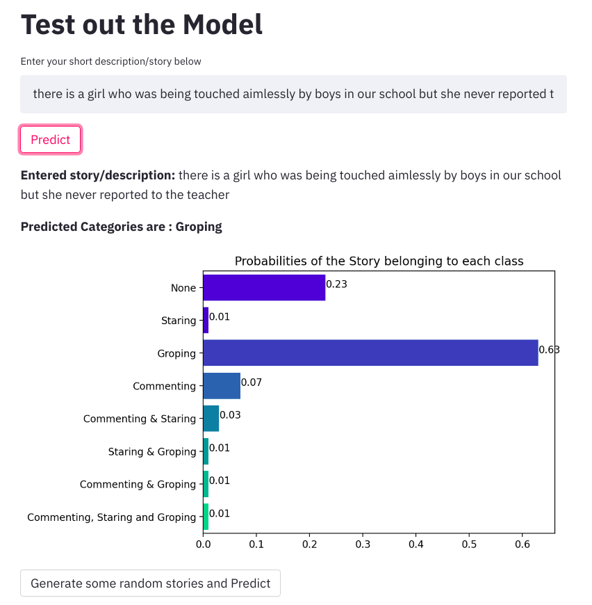
For the development of the frontend, we have used the Streamlit library which makes the process of developing UI for ML apps simpler and intuitive. You can find the link below along with the Github repo of the project.

Link: https://safe-city-clf.herokuapp.com/
Github Repo: https://github.com/AshishSalaskar1/Safe-City-Classification

Future Scope

• In this particular case study, we have tried to focus on employing several Machine Learning models to accomplish our tasks. We can use Deep Learning techniques to build relatively complex models and try to experiment with them.
• For converting text to numerical representations we are using TF-IDF weighted Glove vectors, instead, we can try out more advanced techniques like Fast-Text as well using Deep Learning models like BERT to get a numerical representation of the text.
• The model we have built is trained on samples gathered from Safecity data. So it would be more appropriate to be used on stories submitted on the Safecity website. We can try to use web-scraping to collect more data from similar sites which would help us gather more data and train more complex models on it.

References

• Safecity : https://www.safecity.in/
• SafeCity Dataset

Ashish Salaskar 16 Jul 2021