The Mathematics Behind Support Vector Machine Algorithm (SVM)

This article was published as a part of the Data Science Blogathon.

Introduction

One of the classifiers that we come across while learning about machine learning is Support Vector Machine or SVM. This algorithm is one of the most popular classification algorithms used in machine learning.

In this article, we will learn about the mathematics involved behind the Support Vector Machine for a classification problem, how it classifies the classes and gives a prediction.

1. Support Vector Machine

A Support Vector Machine or SVM is a machine learning algorithm that looks at data and sorts it into one of two categories.

Support Vector Machine is a supervised and linear Machine Learning algorithm most commonly used for solving classification problems and is also referred to as Support Vector Classification.

There is also a subset of SVM called SVR which stands for Support Vector Regression which uses the same principles to solve regression problems.

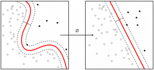
SVM is most commonly used and effective because of the use of the Kernel method which basically helps in solving the non-linearity of the equation in a very easy manner.

P.S. — Since this article is written focusing on the mathematical part. Kindly refer to this article for a complete overview of the working of the algorithm

2. Quintessential Topics for SVM

Support Vector Machine basically helps in sorting the data into two or more categories with the help of a boundary to differentiate similar categories.

So, first let’s revise the formulae for how each data is represented in space, and what is an equation of a line which will help in segregating the similar categories, and lastly the distance formula between a data point and the line (a boundary separating the categories).

2.1 A point in a space

Let’s assume we have some data where we(algorithm of SVM) are asked to differentiate between the males and females based on first studying the characteristics of both the genders and then accurately label the unseen data if someone is a male or a female.

In this example, the characteristics which will help to differentiate the gender are basically called features in machine learning.

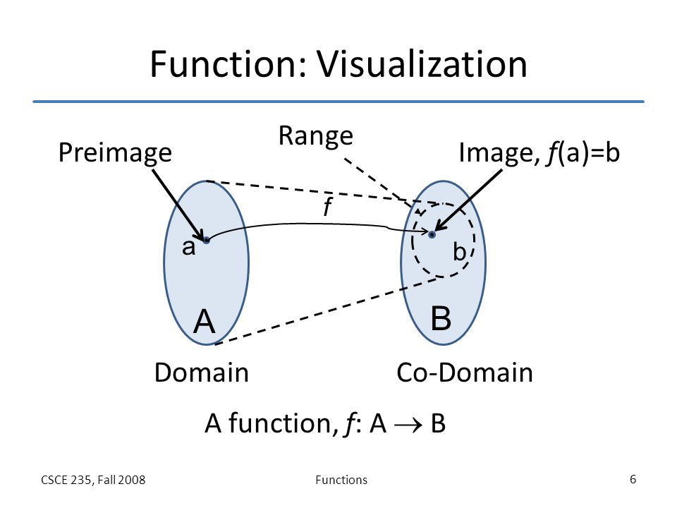
Assuming that we are already familiar with the concept of the domain, range, and co-domain while defining a function in real space. (If not, kindly click on the image for understanding the concept with an example)

When we define x in a real space, we understand its domain, and on mapping a function for y = f(x), we get range and co-domain.

So, initially, we are given the data which is to be separated by the algorithm.

The data given for separating/classifying is represented as a unique point in a space where each point is represented by some feature vector x.

x ∊ R^D

Note: R^D here is a vector space with D dimension, it isn’t necessary to have a hang of this concept for this algorithm.

We are applying a similar concept of the domain, range, mapping a function for the data points here, instead of real space, we have a vector space for x.

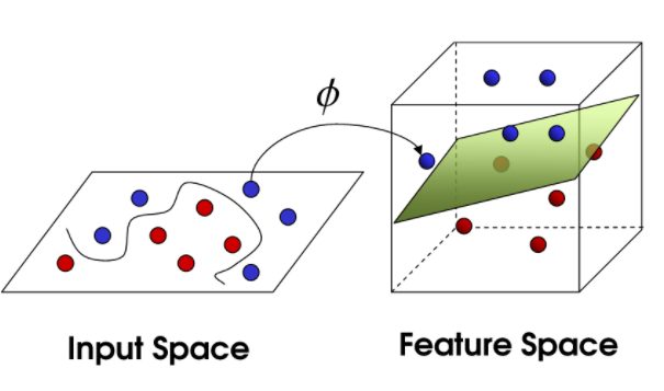
Further, mapping the point on a complex feature space x,

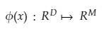
Φ(x) ∊ R^M

The transformed feature space for each input feature mapped to a transformed basis vector Φ(x) can be defined as:

2.2 Decision Boundary

So now that we have represented our points visually, our next job is to separate these points using a line and this is where the term decision boundary comes into the picture.

Decision Boundary is the main separator for dividing the points into their respective classes.

(How and why do I say, main separator and not just any separator will we cover while understanding the math)

Equation of Hyperplane :

The equation of the main separator line is called a hyperplane equation.

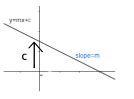
Let us look at the equation for a straight line with slope m and intercept c.

The equation becomes : mx + c = 0

(To notice: we have fit a straight/linear line which is 1-D in a  2-D space)

The hyperplane equation dividing the points (for classifying) can now easily be written as:

H: w^T(x) + b = 0

Here: b = Intercept and bias term of the hyperplane equation

In D dimensional space, the hyperplane would always be D -1 operator.

For example, for 2-D space, a hyperplane is a straight line (1-D).

2.3 Distance Measure

Now that we have seen, how to represent data points, and how to fit a separating line between the points. But, while fitting the separating line, we would obviously want such a line that would be able to segregate the data points in the best possible way having the least mistakes/errors of miss-classification.

So, to have the least errors in the classification of the data points, that concept will require us to first know the distance between a data point and the separating line.

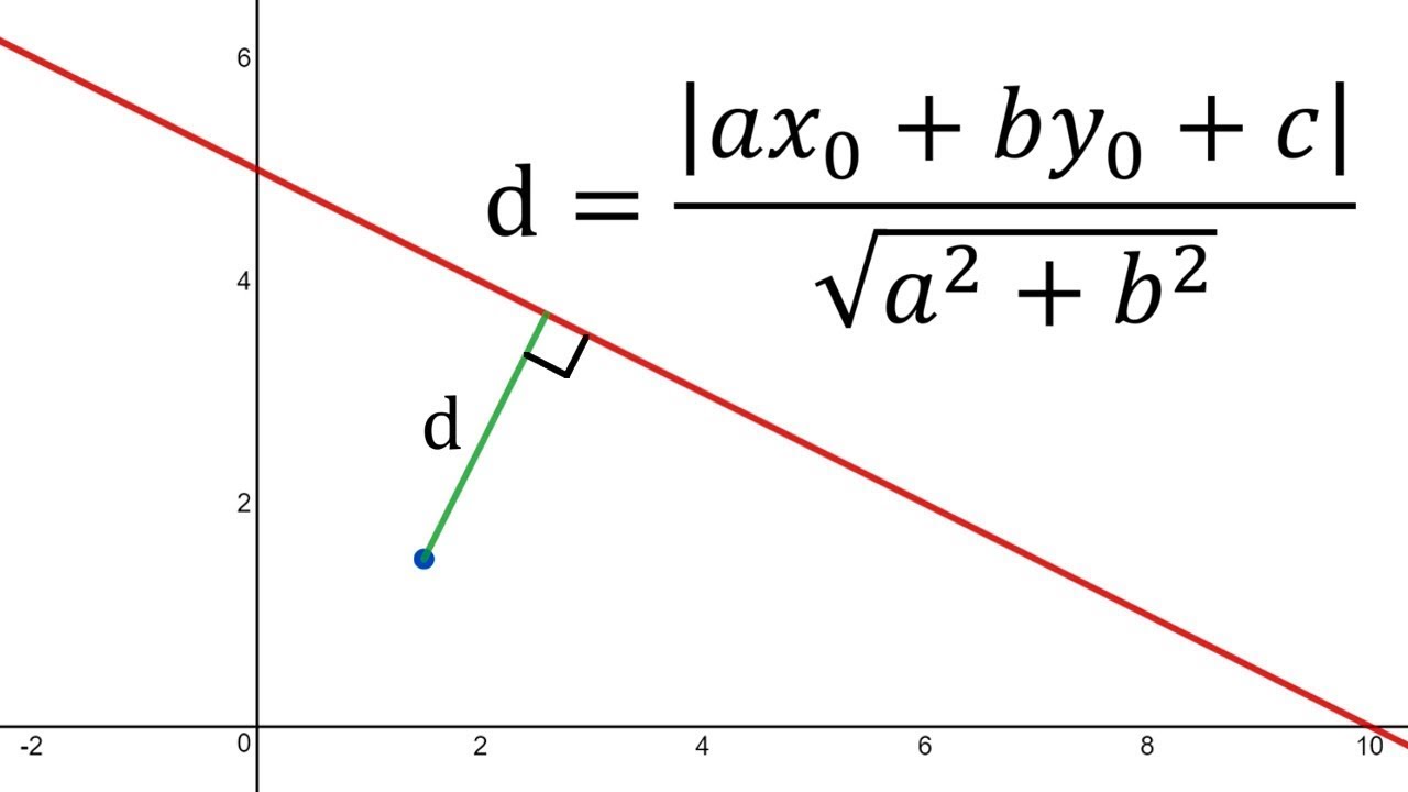
The distance of any line, ax + by + c = 0 from a given point say, (x₀ , y₀) is given by d.

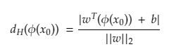
Similarly, the distance of a hyperplane equation: w^TΦ(x) + b = 0 from a given point vector Φ(x₀) can be easily written as :

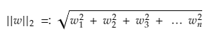
here ||w||2 is the Euclidean norm for the length of w given by :

3. There’s plenty of fish Mathematics in the sea

3.1 Background

We talked about an example of differentiating genders, so such problems are called classification problems. Now a classification problem can have only two (binary) classes for separating or can have more than two too which are known as a multi-class classification problems.

But not all classification predictive models support multi-class classification, algorithms such as the Logistic Regression and Support Vector Machines (SVM) were designed for binary classification and do not natively support classification tasks with more than two classes.

But if someone stills want to use the binary classification algorithms for multi-classification problems, one approach which is widely used is to split the multi-class classification datasets into multiple binary classification datasets and then fit a binary classification model on each.

Two different examples of this approach are the One-vs-Rest and One-vs-One strategies. One can read about the two approaches here.

Moving ahead with the main topic of understanding the math, we  will be considering binary-class classification problem for two reasons:

1. As already mentioned above, SVM works much better for binary class
2.  It would be easy to understand the math since our target variable ( variable / unseen data targeted to predict, whether the point is a male or a female)
3. Note: This will be a One Vs One approach.

3.1.1 Case 1: (Perfect Separation for Binary Classified data) –

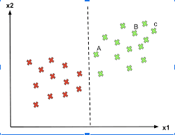
Continuing with our example, if the hyperplane will be able to differentiate between males and females perfectly without doing any miss-classification, then that case of separation is known as Perfect Separation.

Here, in the figure, if males are green and females are red and we can see that the hyperplane which is a line here has perfectly differentiated the two classes.

To generalize, data has two classifications, positive and negative group, and is perfectly separable, meaning that, a hyperplane can accurately separate the *training classes*.

**

(Training data — Data through which algorithm/model learns the pattern on how to differentiate by looking at the features
Testing data — After the model is trained on training data, the model is asked to predict the values for unseen data where only the features are given, and now the model will tell whether its a male or a female)

**

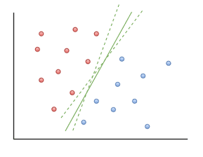
Now, there could be many hyperplanes giving 100% accuracy, as seen in the photograph.

“” So to choose the optimal/best hyperplane, place the hyperplane right at the center where the distance is maximum from the closest points and give the least test errors further. “”

To notice: We have to aim at the least TEST errors and NOT TRAINING errors.

So, we have to maximize the distance to give some space to the hyperplane equation which is also the goal / main idea behind SVM.

The goal of the algorithm involved behind SVM:

So now we have to:

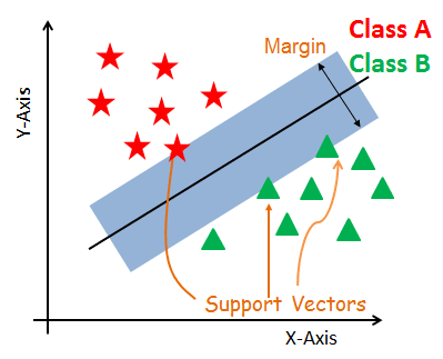
Finding a hyperplane with the maximum margin (margin is basically a protected space around hyperplane equation) and algorithm tries to have maximum margin with the closest points (known as support vectors).

In other words, “The goal is to maximize the minimum distance.”  for the distance (mentioned earlier in section 2)

, given by:

So, now that the goal is understood. While making the predictions on the training data which were binary classified as positive and negative groups, if the point is substituted from the positive group in the hyperplane equation, we will get a value greater than 0 (zero), Mathematically,

w^T(Φ(x)) + b > 0

And predictions from the negative group in the hyperplane equation would give negative value as

w^T(Φ(x)) + b < 0. 

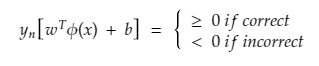
But here the signs were about training data, which is how we are training our model. That for positive class, give a positive sign and for negative give a negative sign.

But while testing this model on test data, If we predict a positive class (positive sign or greater than zero sign) correctly as positive, then two positives makes positive and hence greater than zero result. The same applies if we correctly predict the negative group since two negatives will again make a positive.

But if the model miss classifies the positive group as a negative group then one plus and one minus makes a minus, hence overall less than zero.

Summing up the above concept:

The product of a predicted and actual label would be greater than 0 (zero) on correct prediction, otherwise less than zero.

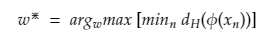
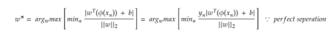
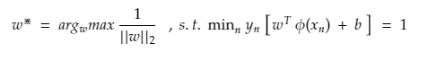
For perfectly separable datasets, the optimal hyperplane classifies all the points correctly, further substituting the optimal values in the weight equation.

Here:

arg max is an abbreviation for arguments of the maxima which are basically the points of the domain of a function at which function values are maximized.

(For further working of arg max in machine learning, do read here.)

Further, bringing the independent term of weight outside gives:

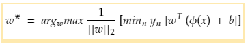
The inner term (min_n y_n |w^T Φ(x) + b | ) basically represents the minimum distance of a point to the decision boundary and the closest point to the decision boundary H.

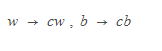
Re-scaling the distance of the closest point as 1 i.e. (min_n y_n |w^T Φ(x) + b |) = 1. Here, the vectors remain in the same direction and the hyperplane equation will not change. It is like changing the scale of a picture; the objects expand or shrink, but the directions remain the same, and the image remains unaltered.

Re-scaling of distance is done by substituting,

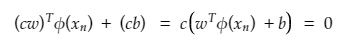
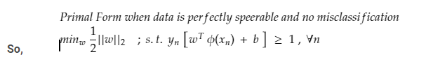
The equation now becomes (describing that every point is at least 1/||w||2 distance apart from hyperplane) as

This maximization problem is equivalent to the following minimization problem which is multiplied by a constant as they don’t affect the results.

3.1.2 Primal Form of SVM (Perfect Separation) :

The above optimization problem is the Primal formulation since the problem statement has original variables.

3.2 CASE 2 : (Non – Perfect Separation)

But we all know, there is no situation where everything is perfect and something always goes the other way around.

In our example of gender classification, we cannot expect the model to give such a hyperplane equation which will perfectly separate both the genders, there would always be one or more than one point which won’t end up in their category while an optimal hyperplane equation is being fit, known as miss classification. (As described in the image below)

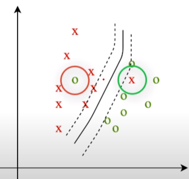
So we can’t expect an ideal/perfect case. Here we become smarter than the model and allow the model to make a few mistakes while classifying the points and therefore,

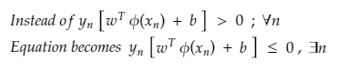
And hence add a slack variable as a penalty for every miss-classification for each data point represented by β (beta). So, no penalty means the data point is correctly classified, β = 0, and at any miss classification β > 1, as a penalty.

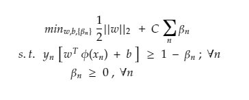
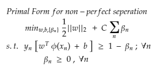
3.2.1 Primal Form of SVM(Non -Perfect Separation):

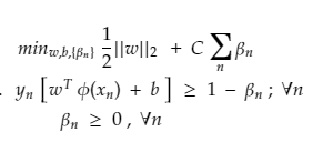
Here: for β and C

Slack for every variable should be as low as possible and further regularized by hyperparameter C

• If C = 0, means less complex boundary as classifier would be not penalized by slack, as a result, the optimum hyperplane can use it anywhere and accept all large misclassifications. And as a result, the decision boundary would be linear and under fitted.

• If C = infinitely high, then even small slacks would be highly penalized and the classifier can't afford to misclassify points and therefore overfitting. So parameter C is important.

The above equation is an example of Convex Quadratic Optimization since the objective function is quadratic in W and constraints are linear in W and β.

Solution for Primal form: (Non – perfect separation):

Since we have Φ, which has a complex notation. we would be rewriting the equation.

Concept is basically to get rid of Φ and hence rewrite Primal formulation in Dual Formulation known as the dual form of a problem and to solve the obtained constraint optimization problem with the help of Lagrange Multiplier method.

In other words :

Dual Form: rewrites the same problem using a different set of variables. So the alternate formulation will help in eliminating the dependence on Φ and reducing the effect will be done with Kernelization.

Lagrange Multiplier Method: It is a strategy to find the local minima or maxima of a function subject to the condition that one or more equations have to be satisfied exactly by the chosen values of variables.

Further, the formal definition of Dual Problem can be defined as :

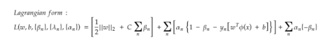
The Lagrangian dual problem is obtained by first forming a Lagrangian of the already obtained minimization problem with the help of a Lagrange Multiplier so that new constraints could be added to the objective function and then would be solved for the primal variable values that minimize the original objective function

This new solution makes the primal variables as functions of the Lagrange multipliers, and are called dual variables so that the new problem is to maximize the objective function for the dual variables with the new derived constraints.

This blog has explained the working of Lagrangian Multipliers in a very good way.

Taking an example of the application of Lagrange multiplier for a better understanding of how to convert a primal formulation using Lagrange multipliers to solve for optimization.

Below x is the original primal variable and to minimize the function f under a set of constraints given by g, and rewriting for a new set of variables called Lagrangian multipliers.

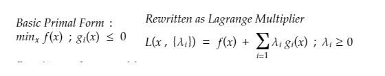
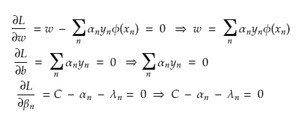
Solving the primal variables by differentiating the unconstrained Lagrange.

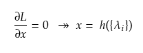
And lastly substituting back in the Lagrange equation and rewriting the constraints

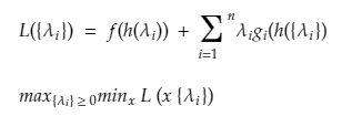
Getting back at our Primal form:

Step 1: Obtain Primal and Determine Lagrangian form from primal

Step 2: Obtaining solution by expressing primal in form of duals

Step 3: Substitute obtained values in the Lagrangian form

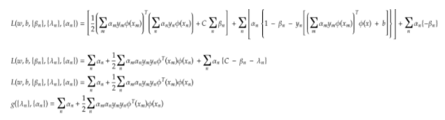
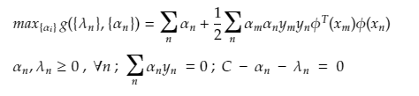
The final dual form from the above simplification is :

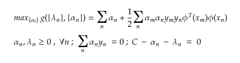
The above dual form still have Φ terms, and here this can be easily solved with the help of Kernelization

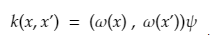
The kernel by definition avoids the explicit mapping that is needed to get linear learning algorithms to learn a nonlinear function or decision boundary For all x and x’ in the input space Φ certain functions k(x,x’) can be expressed as an inner product in another space Ψ. The function

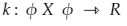
is referred to as a Kernel. In short, for machine learning kernel is defined as written in the form of a “feature map”

which satisfies

For a better understanding of kernels, one can refer to this link of quora

The kernel has two properties:

• It is symmetric in nature k(xn , xm) = k(xm , xn)

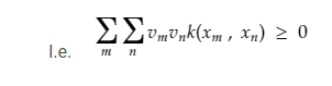
• It is Positive semi-definite

To have an intuition of the working of kernels, this link of quora might be useful.

By the definition of the kernel, we can substitute these values

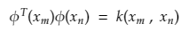
So substituting properties of the kernel and by definition of the kernel in our dual form,

We get The New Equation as :

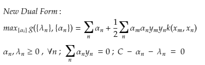
AND this solution is free from Φ and so much easier to compute. And this was the mathematics involved behind the SVM model.

4. Pointing out all the steps mentioned above.

Finally, we are at the end of the article, and to sum up, all the gibber gabber written above

1. Whenever we are given any test feature vector x to predict, mapped to a complex Φ(x) and asked to predict which is basically w^TΦ(x)
2. Then rewrite it using the duals so that the prediction is completely independent of complex feature basis Φ
3. And is further predicted using kernels

4. Hence, concludes that we don’t need a complex basis to model non-separable data well, and the kernel does the job.

Frequently Asked Questions

I hope I was able to cover the basic intuition and mathematics behind SVM, 
for the classifier model, and keeping the length of the article in mind, I have tried to attach all the important links for the corresponding links within the article.

This was my understanding of involved mathematics in SVM,
 and I am open to suggestions regarding my work here

Radhika 19 Jul 2023