Performing Time Series Analysis using ARIMA Model in R
Welcome to the World of Time Series Analysis!
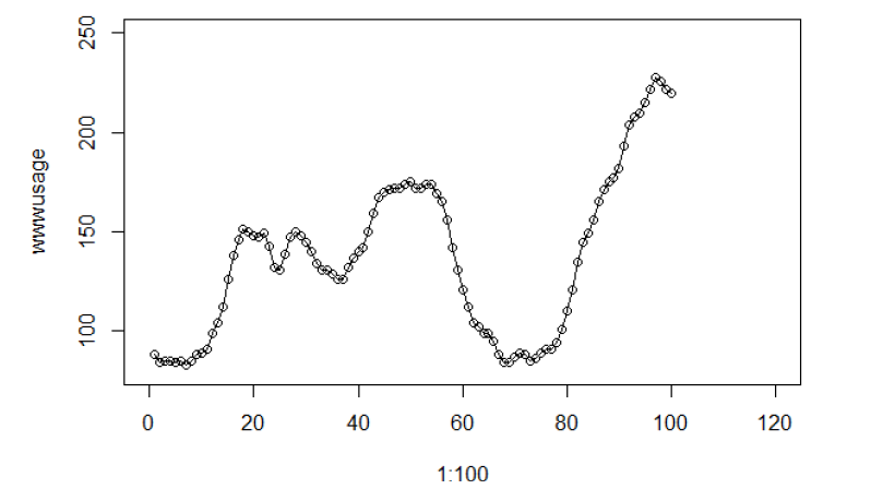
From this article, you will learn how to perform time series analysis using the ARIMA model (with code!). The dataset used in this article can be downloaded here. The usage time series data consist of the number of users connected to the internet through a server. The data are collected at a time interval of one minute and there are 100 observations. I will fit an appropriate ARIMA model for it using R codes.
Stationary Time Series
A key role in time series analysis is played by processes whose properties, or some of them, do not vary over time. Such a property is illustrated in the following important concept, stationarity. We then introduce the most commonly used stationary linear time series models–the autoregressive integrated moving average (ARIMA) models. These models have assumed great importance in modeling real-world processes.
ARIMA in Time Series Analysis
An autoregressive integrated moving average – ARIMA model is a generalization of a simple autoregressive moving average – ARMA model. Both of these models are used to forecast or predict future points in the time-series data. ARIMA is a form of regression analysis that indicates the strength of a dependent variable relative to other changing variables.
The final objective of the model is to predict future time series movement by examining the differences between values in the series instead of through actual values. ARIMA models are applied in the cases where the data shows evidence of non-stationarity. In time series analysis, non-stationary data are always transformed into stationary data.
The common causes of non-stationary in time series data are the trend and the seasonal components. The way to transformed non-stationary data to stationary is to apply the differencing step. It is possible to apply one or more times of differencing steps to eliminate the trend component in the data. Similarly, to remove the seasonal components in data, seasonal differencing could be applied. [1]
According to the name, we can split the model into smaller components as follow:
- AR: an AutoregRegressive model which represents a type of random process. The output of the model is linearly dependent on its own previous value i.e. some number of lagged data points or the number of past observations [2].
- MA: a Moving Average model which output is dependent linearly on the current and various past observations of a stochastic term [3].
- I: integrated here means the differencing step to generate stationary time series data, i.e. removing the seasonal and trend components [1].
ARIMA model is generally denoted as ARIMA(p, d, q) and parameter p, d, q are defined as follow:
- p: the lag order or the number of time lag of autoregressive model AR(p)
- d: degree of differencing or the number of times the data have had subtracted with past value
- q: the order of moving average model MA(q)
Read the dataset
wwwusage = scan("wwwusage.txt", skip=1)
Time series plot
# x-axis show values from 0 to 120 while y-axis show values from 80 to 250 according to min, max values of dataset
plot(1:100, wwwusage, xlim = c(0, 120), ylim=c(80, 250))
#connect the datapoints with line
lines(1:100, wwwusage, type="l")
Interpretation of sample ACF and PACF plot
ACF: The autocorrelation coefficient function, define how the data points in a time series are related to the preceding data points.
PACF: The partial autocorrelation coefficient function, like the autocorrelation function, conveys vital information regarding the dependence structure of a stationary process.
Now let’s explain how to select a model based on ACF and PACF plots.
Given observations of a time series, one approach to the fitting of a model to the data is to match the sample ACF and sample PACF of the data with the ACF and PACF of the model, respectively. We can use the sample ACF plot to see if the specific time series data is stationary or not. Here is an example of how the sample ACF plot will look like if the time series is not stationary.
For stationary time-series data, the sample ACF will die down very quickly or even cuts off. Otherwise, the time series is not stationary. Cut off here means the ACF value is less than the indicated confidence interval or inside the blue dotted line.
If we confirm the data is stationary, we can decide which parameters q and p should be used for the model based on at which lag the sample ACF and PACF value cut off. In this case, parameter p will be decided by sample PACF cut off time and parameter q will be decided by sample ACF cut off time. If we know the time series is not stationary, will try to perform the higher-order differencing to ensure the data is stationary.
Sample ACF and PACF plot
acf(wwwusage, lag.max=100)
pacf(wwwusage, lag.max=100)
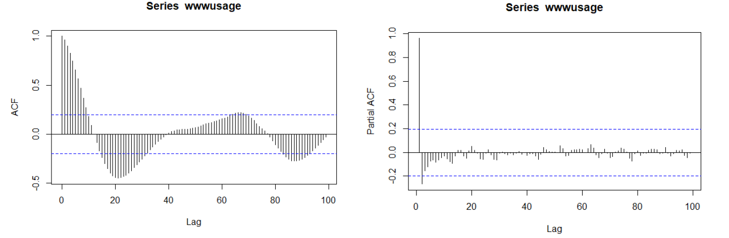
From both time series and sample ACF plot, we get the conclusion that the raw data is not stationary. Sample ACF got the periodical pattern, which very likely contains seasonal components. If data contains trend and seasonal components, it is said to be non-stationary.
Sample PACF cut off after lag 2, however, we can’t use it to decide what model to use since the data is not stationary.
Take first-order differencing
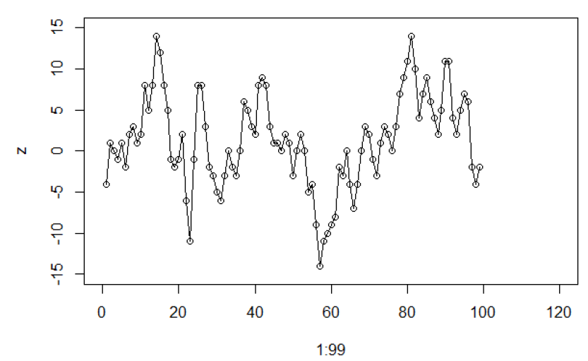
zt = wwwusaget – wwwusaget-1 = (1-B) wwwusaget
z = diff(wwwusage, 1, 1)
plot(1:99, z, xlim = c(0, 120), ylim=c(-15, 15))
lines(1:99, z, type="l" )
acf(z, lag.max=100)
pacf(z, lag.max=100)
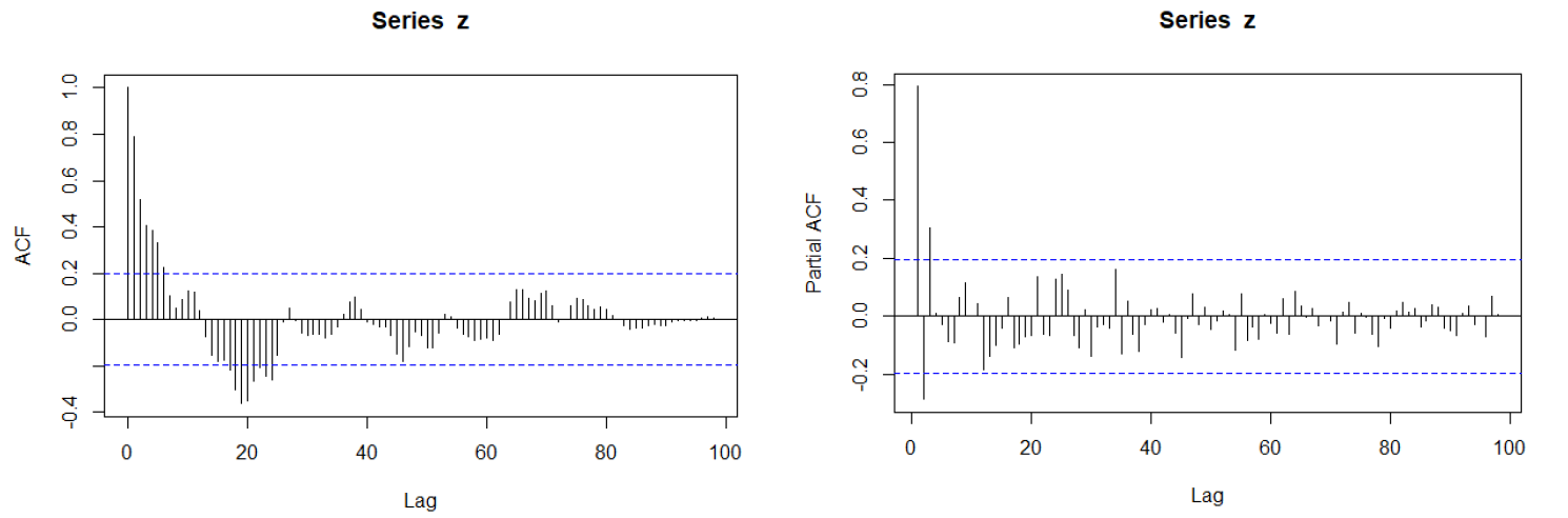
From sample ACF plot, we still can see some periodical pattern, so decided to apply higher-order differencing i.e. second-order differencing on original data. The purpose is to check if higher-order differencing can get a better result.
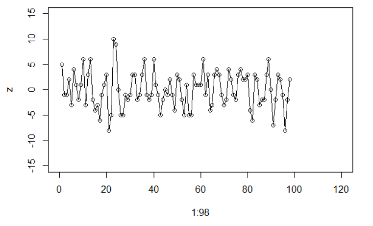
Take second-order differencing
zt = wwwusaget – 2wwwusaget-1 + wwwusaget-2 = (1-2B+B2) wwwusaget
z = diff(wwwusage, 1, 2)
plot(1:98, z, xlim = c(0, 120), ylim=c(-15, 15))
lines(1:98, z, type="l" )
acf(z, lag.max=100)
pacf(z, lag.max=100)
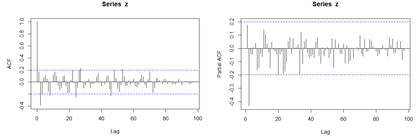
We can see sample ACF decay very fast, so the data is stationary. It is acceptable to have 5% of time lags lie outside the dotted blue boundary. Therefore, we can ignore around 5-time lags (5% x 100) at lag 8, 23, 26, 44, and 52.
Since sample ACF cut off after lag 2, we can use ARIMA(0,2,2) for wwwusage. Similarly, for sample PACF, it cut off after lag 2 we can use ARIMA(2,2,0) for wwwusage.
Model 1: ARIMA(0,2,2)
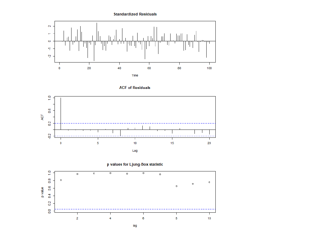
fit1 = arima(wwwusage, order = c(0,2,2))
tsdiag(fit1)
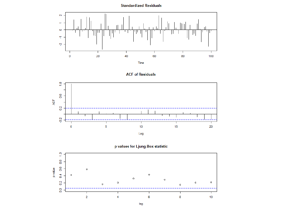
Thus, model 1 is adequate, i.e. there is no autocorrelation in the residuals.
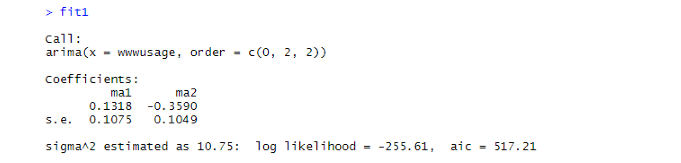
The fitted model is: (1-2B+B2) wwwusaget = zt + 0.1318zt-1 – 0.3590zt-2
Model 2: ARIMA(2,2,0)
fit2 = arima(wwwusage, order = c(2,2,0))
tsdiag(fit2)
Thus, model 2 is adequate, i.e. there is no autocorrelation in the residuals.
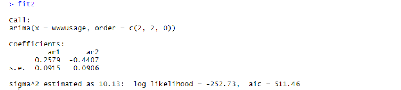
The fitted model is: (1-2B+B2) wwwusaget = 0.2579 wwwusaget-1 – 0.4407 wwwusaget-2 + zt
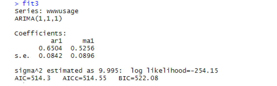
Model 3: Auto ARIMA
library(forecast)
fit3 = auto.arima(wwwusage)
tsdiag(fit3)
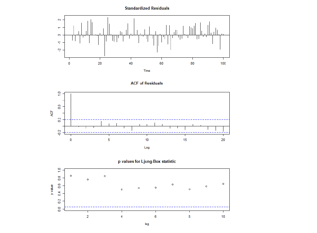
Thus, model 3 is adequate, i.e. there is no autocorrelation in the residuals.
Evaluation based on AIC
|
Model |
AIC criterion |
|
Model 1: ARIMA(0,2,2) |
517.21 |
|
Model 2: ARIMA(2,2,0) |
511.46 |
|
Model 3: ARIMA(1,1,1) |
514.3 |
From the diagnostic checking, all the 3 models are adequate. AIC criterion allowed us to compare the fit of different models if the models are adequate. The smaller the AIC criterion, the better the model. Therefore, a final fitted model chosen for wwwusage data is ARIMA(2,2,0) which give the lowest AIC (511.46) among all models from the table above.
Conclusion
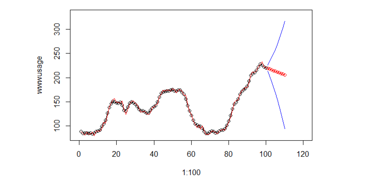
Final fitted model ARIMA(2,2,0) with fitted values and forecast for 10 steps ahead
# fitted values
plot(1:100, wwwusage, xlim = c(0, 120), ylim=c(80, 330))
lines(1:100, wwwusage, type="l" )
lines(1:100, wwwusage-fit2$residuals, type="l", col="red")

# forecast for 10 steps ahead
forecast = predict(fit2, n.ahead=10)
lines(101:110, forecast$pred, type="o", col="red")
lines(101:110, forecast$pred-1.96*forecast$se, col="blue")
lines(101:110, forecast$pred+1.96*forecast$se, col="blue")
References
[1] Autoregressive integrated moving average – Wikipedia
[2] Autoregressive model – Wikipeida
[3] Moving average model -Wikipedia
About the Author
Here is my profile on LinkedIn.
Thanks for giving your time!


