A Guide to Building an End-to-End Multiclass Text Classification Model

Introduction

Knock! Knock! Who’s there? It’s Natural Language Processing!

Natural language processing (NLP) is everywhere, one of the most used concepts in the business world. Whether to predict the sentiment in a sentence or to differentiate the emails, or flag a toxic comment, all these scenarios use a strong natural language processing concept called text classification. I can understand in the above cases, we have a maximum target class of two or three. Can we go beyond that? Can we build a multiclass text classification model? Well! Yes, we can do it.

Today, we will implement a multiclass text classification model on an open-source dataset and explore more about the steps and procedure. Let’s begin.

Learning Objectives

1. Understand the importance of Natural Language Processing (NLP) in text classification and its applications in real-world scenarios.
2. Learn the process of building an end-to-end multiclass text classification model, from loading the dataset to evaluating model performance.
3. Explore feature engineering techniques, such as text processing and TF-IDF vectorization, for transforming textual data into a suitable format for machine learning models.
4. Compare and contrast the performance of various classification algorithms, including Linear Support Vector Machine, Random Forest, Multinomial Naive Bayes, and Logistic Regression.
5. Gain hands-on experience with implementing a multiclass text classification model using Python, pandas, scikit-learn, and other relevant libraries, while understanding the challenges and considerations involved in the process.

This article was published as a part of the Data Science Blogathon.

Dataset for Text Classification

The dataset which we are going to use is available publicly, and it is quite a huge dataset. It consists of complaints received from the consumer regarding the products and services. The dataset is available here (https://catalog.data.gov/dataset/consumer-complaint-database).

The dataset consists of real-world complaints received from customers regarding financial products and services. The complaints are labeled to a specific product. Hence, we can conclude that this is a supervised problem statement, where we have the input and the target output for that. We will play with different machine learning algorithms and check which algorithm works better.

We aim to classify the complaints of the consumer into predefined categories using a suitable classification algorithm. For now, we will be using the following classification algorithms.

• Linear Support Vector Machine (LinearSVM)
• Random Forest
• Multinomial Naive Bayes
• Logistic Regression.

Loading the Data

Download the dataset from the link given in the above section. Since I am using Google Colab, if you want to use the same, you can use the Google Drive link given here and import the dataset from your Google Drive. The below code will mount the drive and unzip the data to the current working directory in Colab.

from google.colab import drive
drive.mount('/content/drive')
!unzip /content/drive/MyDrive/rows.csv.zip

First, we will install the required modules.

• Pip install numpy
• Pip install pandas
• Pip install seaborn
• Pip install scikit-learn
• Pip install scipy

Once everything is successfully installed, we will import the required libraries.

import os
import pandas as pd
import numpy as np
from scipy.stats import randint
import seaborn as sns # used for plot interactive graph.
import matplotlib.pyplot as plt
import seaborn as sns
from io import StringIO
from sklearn.feature_extraction.text import TfidfVectorizer
from sklearn.feature_selection import chi2
from IPython.display import display
from sklearn.model_selection import train_test_split
from sklearn.feature_extraction.text import TfidfTransformer
from sklearn.naive_bayes import MultinomialNB
from sklearn.linear_model import LogisticRegression
from sklearn.ensemble import RandomForestClassifier
from sklearn.svm import LinearSVC
from sklearn.model_selection import cross_val_score
from sklearn.metrics import confusion_matrix
from sklearn import metrics

Now, after this, let us load the dataset and see the shape of the loaded dataset.

# loading data
df = pd.read_csv('/content/rows.csv')
print(df.shape)

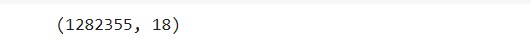
From the output of the above code, we can say that the dataset is very huge, and it has 18 columns. Let us see what the data looks like. Execute the code below.

df.head(3).T

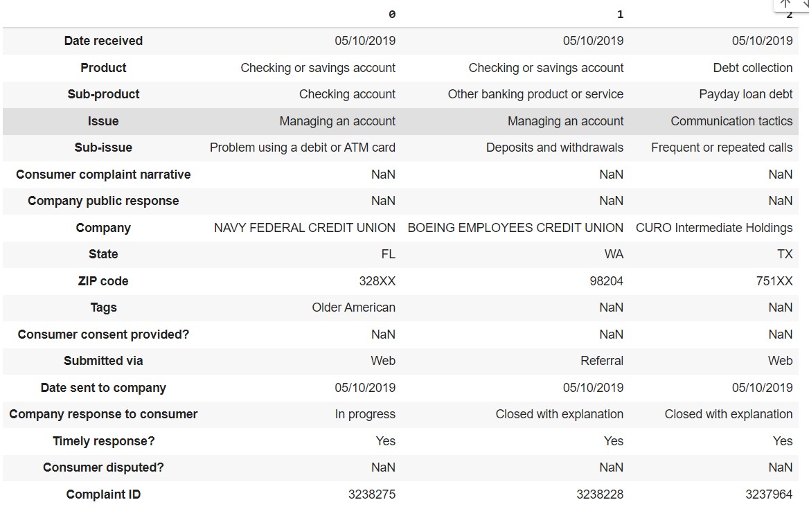
Now, for our multi-class text classification task, we will be using only two of these columns out of 18, that is, the column with the name ‘Product’ and the column ‘Consumer complaint narrative’. Now let us create a new DataFrame to store only these two columns, and since we have enough rows, we will remove all the missing (NaN) values. To make it easier to understand, we will rename the second column of the new DataFrame as ‘consumer_complaints’.

# Create a new dataframe with two columns
df1 = df[['Product', 'Consumer complaint narrative']].copy()
# Remove missing values (NaN)
df1 = df1[pd.notnull(df1['Consumer complaint narrative'])]
# Renaming second column for a simpler name
df1.columns = ['Product', 'Consumer_complaint']
print(df1.shape)
df1.head(3).T

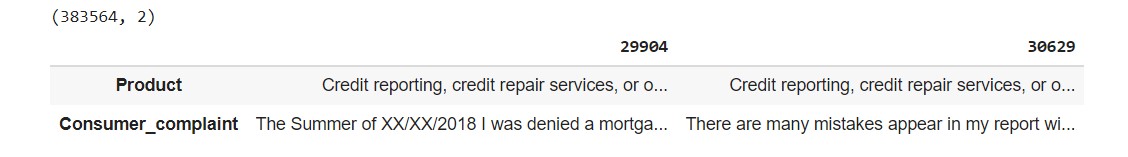
We can see that after discarding all the missing values, we have around 383k rows and 2 columns; this will be our data for training. Now let us check how many unique products there are.

pd.DataFrame(df1.Product.unique()).values

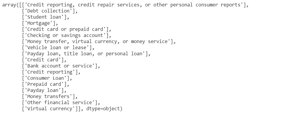
There are 18 categories in products. To make the training process easier, we will do some changes in the names of the category.

# Because the computation is time consuming (in terms of CPU), the data was sampled
df2 = df1.sample(10000, random_state=1).copy()
# Renaming categories
df2.replace({'Product': 
             {'Credit reporting, credit repair services, or other personal consumer reports': 
              'Credit reporting, repair, or other', 
              'Credit reporting': 'Credit reporting, repair, or other',
             'Credit card': 'Credit card or prepaid card',
             'Prepaid card': 'Credit card or prepaid card',
             'Payday loan': 'Payday loan, title loan, or personal loan',
             'Money transfer': 'Money transfer, virtual currency, or money service',
             'Virtual currency': 'Money transfer, virtual currency, or money service'}}, 
            inplace= True)
pd.DataFrame(df2.Product.unique())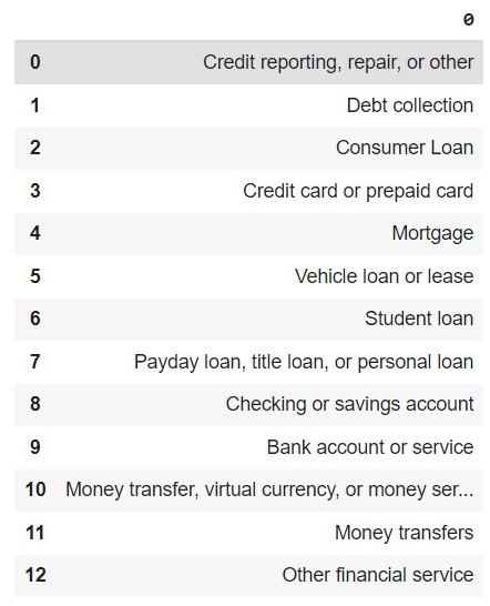

The 18 categories are now reduced to 13; we have combined ‘Credit Card’ and ‘Prepaid card’ into a single class, and so on.

Now, we will map each of these categories to a number, so that our model can understand it in a better way and we will save this in a new column named ‘category_id’. Where each of the 12 categories is represented numerically.

# Create a new column 'category_id' with encoded categories 
df2['category_id'] = df2['Product'].factorize()[0]
category_id_df = df2[['Product', 'category_id']].drop_duplicates()
# Dictionaries for future use
category_to_id = dict(category_id_df.values)
id_to_category = dict(category_id_df[['category_id', 'Product']].values)
# New dataframe
df2.head()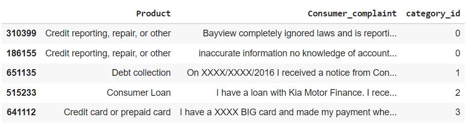

Let us visualize the data and see how many numbers of complaints there are per category. We will use a Bar chart here.

fig = plt.figure(figsize=(8,6))
colors = ['grey','grey','grey','grey','grey','grey','grey','grey','grey',
    'grey','darkblue','darkblue','darkblue']
df2.groupby('Product').Consumer_complaint.count().sort_values().plot.barh(
    ylim=0, color=colors, title= 'NUMBER OF COMPLAINTS IN EACH PRODUCT CATEGORYn')
plt.xlabel('Number of ocurrences', fontsize = 10);

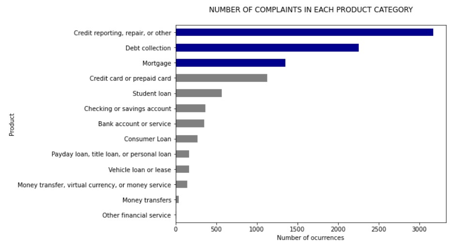
The above graph shows that most of the customers complained about:

• Credit reporting, repair, or other
• Debt collection
• Mortgage

Text processing

The text needs to be preprocessed so that we can feed it to the classification algorithm. Here we will transform the texts into vectors using Term Frequency-Inverse Document Frequency (TFIDF) and evaluate how important a particular word is in the collection of words. For this, we need to remove punctuations and do lower casing, and then the word importance is determined in terms of frequency.

We will be using the TfidfVectorizer function with the below parameters:

• min_df: remove the words that have occurred in less than the ‘min_df’ number of files.
• Sublinear_tf: if True, then scale the frequency in logarithmic scale.
• Stop_words: it removes stop words which are predefined in ‘english’.

tfidf = TfidfVectorizer(sublinear_tf=True, min_df=5,
                        ngram_range=(1, 2), 
                        stop_words='english')
# We transform each complaint into a vector
features = tfidf.fit_transform(df2.Consumer_complaint).toarray()
labels = df2.category_id
print("Each of the %d complaints is represented by %d features (TF-IDF score of unigrams and bigrams)" %(features.shape))

Now, we will find the most correlated terms with each of the defined product categories. Here, we are finding only the three most correlated terms.

# Finding the three most correlated terms with each of the product categories
N = 3
for Product, category_id in sorted(category_to_id.items()):
  features_chi2 = chi2(features, labels == category_id)
  indices = np.argsort(features_chi2[0])
  feature_names = np.array(tfidf.get_feature_names())[indices]
  unigrams = [v for v in feature_names if len(v.split(' ')) == 1]
  bigrams = [v for v in feature_names if len(v.split(' ')) == 2]
  print("n==> %s:" %(Product))
  print("  * Most Correlated Unigrams are: %s" %(', '.join(unigrams[-N:])))
  print("  * Most Correlated Bigrams are: %s" %(', '.join(bigrams[-N:])))

The output will be like this: for each category, it will show the three most correlated terms. We can find any number of correlated terms per category; in the above code, the value of ‘N’ is set to 3, which means it will display the 3 most correlated terms; feel free to change the number and check all the terms are highly correlated. But for this small task, to know which terms have more weightage, we will see the top three correlated terms.

==> Bank account or service:
  * Most Correlated Unigrams are: overdraft, bank, scottrade
  * Most Correlated Bigrams are: citigold checking, debit card, checking account

==> Checking or savings account:
  * Most Correlated Unigrams are: checking, branch, overdraft
  * Most Correlated Bigrams are: 00 bonus, overdraft fees, checking account

==> Consumer Loan:
  * Most Correlated Unigrams are: dealership, vehicle, car
  * Most Correlated Bigrams are: car loan, vehicle loan, regional acceptance

==> Credit card or prepaid card:
  * Most Correlated Unigrams are: express, citi, card
  * Most Correlated Bigrams are: balance transfer, american express, credit card

==> Credit reporting, repair, or other:
  * Most Correlated Unigrams are: report, experian, equifax
  * Most Correlated Bigrams are: credit file, equifax xxxx, credit report

==> Debt collection:
  * Most Correlated Unigrams are: collect, collection, debt
  * Most Correlated Bigrams are: debt collector, collect debt, collection agency

==> Money transfer, virtual currency, or money service:
  * Most Correlated Unigrams are: ethereum, bitcoin, coinbase
  * Most Correlated Bigrams are: account coinbase, coinbase xxxx, coinbase account

==> Money transfers:
  * Most Correlated Unigrams are: paypal, moneygram, gram
  * Most Correlated Bigrams are: sending money, western union, money gram

==> Mortgage:
  * Most Correlated Unigrams are: escrow, modification, mortgage
  * Most Correlated Bigrams are: short sale, mortgage company, loan modification

==> Other financial service:
  * Most Correlated Unigrams are: meetings, productive, vast
  * Most Correlated Bigrams are: insurance check, check payable, face face

==> Payday loan, title loan, or personal loan:
  * Most Correlated Unigrams are: astra, ace, payday
  * Most Correlated Bigrams are: 00 loan, applied payday, payday loan

==> Student loan:
  * Most Correlated Unigrams are: student, loans, navient
  * Most Correlated Bigrams are: income based, student loan, student loans

==> Vehicle loan or lease:
  * Most Correlated Unigrams are: honda, car, vehicle
  * Most Correlated Bigrams are: used vehicle, total loss, honda financial

Exploring Multi-classification (classifier) Models

The classification models that we are using:

• Random Forest
• Linear Support Vector Machine
• Multinomial Naive Bayes
• Logistic Regression.

You can refer to their official guide for more information regarding each model.

Now, we will split the data into train and test sets. We will use 75% of the data for training and the rest for testing. Column ‘consumer_complaint’ will be our X or the input, and the product is our Y or the output.

X = df2['Consumer_complaint'] # Collection of documents
y = df2['Product'] # Target or the labels we want to predict (i.e., the 13 different complaints of products)
X_train, X_test, y_train, y_test = train_test_split(X, y, 
                                                    test_size=0.25,
                                                    random_state = 0)

We will keep all the models in a list and loop through the list for each model to get a mean accuracy and standard deviation to calculate and compare the performance for each of these models. Then, we can decide with which model we can move further.

models = [
    RandomForestClassifier(n_estimators=100, max_depth=5, random_state=0),
    LinearSVC(),
    MultinomialNB(),
    LogisticRegression(random_state=0),
]
# 5 Cross-validation
CV = 5
cv_df = pd.DataFrame(index=range(CV * len(models)))
entries = []
for model in models:
  model_name = model.__class__.__name__
  accuracies = cross_val_score(model, features, labels, scoring='accuracy', cv=CV)
  for fold_idx, accuracy in enumerate(accuracies):
    entries.append((model_name, fold_idx, accuracy))
cv_df = pd.DataFrame(entries, columns=['model_name', 'fold_idx', 'accuracy'])

The above code will take some time to complete its execution.

Compare Text Classification Model performance

Here, we will compare the ‘Mean Accuracy’ and ‘Standard Deviation for each classification algorithm.

mean_accuracy = cv_df.groupby('model_name').accuracy.mean()
std_accuracy = cv_df.groupby('model_name').accuracy.std()

acc = pd.concat([mean_accuracy, std_accuracy], axis= 1, 
          ignore_index=True)
acc.columns = ['Mean Accuracy', 'Standard deviation']
acc

From the above table, we can clearly say that the Linear Support Vector Machine’ outperforms all the other classification algorithms. So, we will use LinearSVC to train model multi-class text classification tasks.

plt.figure(figsize=(8,5))
sns.boxplot(x='model_name', y='accuracy', 
            data=cv_df, 
            color='lightblue', 
            showmeans=True)
plt.title("MEAN ACCURACY (cv = 5)n", size=14);

Evaluation of Multiclass Text Classification Model

Now, let us train our model using ‘Linear Support Vector Machine’, so that we can evaluate and check its performance on unseen data.

X_train, X_test, y_train, y_test,indices_train,indices_test = train_test_split(features,labels, df2.index, test_size=0.25,random_state=1)
model = LinearSVC()
model.fit(X_train, y_train)
y_pred = model.predict(X_test)

We will generate a classification report to get more insights into model performance.

# Classification report
print('ttttCLASSIFICATIION METRICSn')
print(metrics.classification_report(y_test, y_pred, 
                                    target_names= df2['Product'].unique()))

From the above classification report, we can observe that the classes that have a greater number of occurrences tend to have a good f1-score compared to other classes. The categories which yield better classification results are ‘Student loan,’ ‘Mortgage,’ and ‘Credit reporting, repair, or other.’ The classes like ‘Debt collection’ and ‘credit card or prepaid card’ can also give good results. Now, let us plot the confusion matrix to check the misclassified predictions.

conf_mat = confusion_matrix(y_test, y_pred)
fig, ax = plt.subplots(figsize=(8,8))
sns.heatmap(conf_mat, annot=True, cmap="Blues", fmt='d',
            xticklabels=category_id_df.Product.values, 
            yticklabels=category_id_df.Product.values)
plt.ylabel('Actual')
plt.xlabel('Predicted')
plt.title("CONFUSION MATRIX - LinearSVCn", size=16);

From the above confusion matrix, we can say that the model is doing a pretty decent job. It has classified most of the categories accurately.

Prediction for the Machine Learning Model

Let us make some predictions on the unseen data and check the model performance.

X_train, X_test, y_train, y_test = train_test_split(X, y, 
                                                    test_size=0.25,
                                                    random_state = 0)
tfidf = TfidfVectorizer(sublinear_tf=True, min_df=5,
                        ngram_range=(1, 2), 
                        stop_words='english')

fitted_vectorizer = tfidf.fit(X_train)
tfidf_vectorizer_vectors = fitted_vectorizer.transform(X_train)
model = LinearSVC().fit(tfidf_vectorizer_vectors, y_train)

Now run the prediction.

complaint = """I have received over 27 emails from XXXX XXXX who is a representative from Midland Funding LLC. 
From XX/XX/XXXX I received approximately 6 emails. From XX/XX/XXXX I received approximately 6 emails. 
From XX/XX/XXXX I received approximately 9 emails. From XX/XX/XXXX I received approximately 6 emails. 
All emails came from the same individual, XXXX XXXX. It is becoming a nonstop issue of harassment."""
print(model.predict(fitted_vectorizer.transform([complaint])))

complaint = """Respected Sir/ Madam, I am exploring the possibilities for financing my daughter 's 
XXXX education with private loan from bank. I am in the XXXX on XXXX visa. 
My daughter is on XXXX dependent visa. As a result, she is considered as international student. 
I am waiting in the Green Card ( Permanent Residency ) line for last several years.
I checked with Discover, XXXX XXXX websites. While they allow international students to apply for loan, they need cosigners who are either US citizens or Permanent Residents. I feel that this is unfair.
I had been given mortgage and car loans in the past which I closed successfully. I have good financial history. 
I think I should be allowed to remain cosigner on the student loan. I would be much obliged if you could look into it. Thanking you in advance. Best Regards"""
print(model.predict(fitted_vectorizer.transform([complaint])))

complaint = """They make me look like if I was behind on my Mortgage on the month of XX/XX/2018 & XX/XX/XXXX when I was not and never was, when I was even giving extra money to the Principal.
The Money Source Web site and the managers started a problem, when my wife was trying to increase the payment, so more money went to the Principal and two payments came out that month and because
I reverse one of them thru my Bank as Fraud they took revenge and committed slander against me by reporting me late at the Credit Bureaus, for 45 and 60 days, when it was not thru. Told them to correct that and the accounting department or the company revert that letter from going to the Credit Bureaus to correct their injustice. The manager by the name XXXX requested this for the second time and nothing yet. I am a Senior of XXXX years old and a Retired XXXX Veteran and is a disgraced that Americans treat us that way and do not want to admit their injustice and lies to the Credit Bureau."""
print(model.predict(fitted_vectorizer.transform([complaint])))

The model is not perfect, yet it is performing very good.

The notebook is available here.

Conclusion

In conclusion, this tutorial demonstrated how to build a sophisticated multiclass text classification model using Python, a cornerstone of data science and deep learning. It highlighted the crucial role of preprocessing and the effectiveness of TF-IDF vectorization in text analysis. The guide touched upon the challenges of imbalanced datasets and introduced neural networks and embedding techniques, including BERT, as advanced solutions for capturing deep semantic relationships in text.

Leveraging TensorFlow and Keras, we showcased the practical application of these deep learning frameworks in enhancing text classification. Although specifics like epochs, batch_size, and encoding functions were not detailed, their importance in optimizing model training cannot be overstated.

This tutorial serves as a testament to the power of Python in simplifying the implementation of complex algorithms for NLP tasks. It underscores the synergy between deep learning and NLP, offering insights into the future of automated text analysis and the potential for further advancements in the field.

Key Takeaways

1. Importance of NLP in Business: Natural Language Processing (NLP) is widely used in the business world, with text classification being a crucial concept. It is employed in scenarios such as sentiment prediction, email differentiation, and identifying toxic comments.
2. Multi-Class Text Classification: The blog focuses on building a multi-class text classification model, demonstrating that it’s possible to classify text into more than two or three categories. In this case, a dataset of consumer complaints regarding financial products and services is used for training.
3. Dataset Preparation: The dataset is loaded, and relevant columns are selected for the multi-class text classification task. The target classes are predefined products, and preprocessing steps involve handling missing values and renaming columns for clarity.
4. Model Comparison: Four classification algorithms (Linear Support Vector Machine, Random Forest, Multinomial Naive Bayes, Logistic Regression) are compared for performance using cross-validation. Linear Support Vector Machine is identified as the top-performing model for this task.
5. Model Evaluation: The Linear Support Vector Machine model is trained and evaluated on unseen data. The classification report and confusion matrix provide insights into the model’s performance, indicating good accuracy and appropriate handling of various product categories.

Frequently Asked Questions

The media shown in this article is not owned by Analytics Vidhya and are used at the Author’s discretion

Syed Abdul Gaffar Shakhadri 19 Feb 2024

I am an enthusiastic AI developer, I love playing with different problems and building solutions.