


Many enterprise data science teams are using Cloudera’s machine learning platform for model exploration and training, including the creation of deep learning models using Tensorflow, PyTorch, and more. However, training a deep learning model is often a time-consuming process, thus GPU and distributed model training approaches are employed to accelerate the training speed.
This is the first post of our blog series on distributed model training for deep learning on Cloudera’s machine learning platform, including both Cloudera Data Science Workbench (CDSW) and Cloudera Machine Learning (CML), a new generation of CDSW built for the cloud. Hereafter for simplicity we’ll refer to only “CML”, but the blog’s contents apply to CDSW installations as well.
In this post, we will present:
- Basic methods of distributed model training for deep learning
- Approaches of how to integrate these methods into CML
- New functionality that automates the parameter server-based distributed Tensorflow model training
- And a preview of enabling MPI Allreduce distributed model training using upcoming CML functionality.
Technical fundamentals on distributed model training for deep learning
Deep learning models are generally trained using the stochastic gradient descendent (SGD) algorithm. For each iteration of SGD, we will sample a mini-batch from the training set, feed it into the training model, calculate the gradient of the loss function of the observed values and the real values, and update the model parameters (or weights). As it is well known that the SGD iterations have to be executed sequentially, it is not possible to speed up the training process by parallelizing iterations. However, as processing one single iteration for a number of commonly used models like CIFAR10 or IMAGENET takes a long time, even using the most sophisticated GPU, we can still try to parallelize the feedforward computation as well as the gradient calculation within each iteration to speed up the model training process.
In practice, we will split the mini-batch of the training data into several parts, like 4, 8, 16, etc. (in this article, we will use the term sub-batch to refer to these split parts), and each training worker takes one sub-batch. Then the training workers do feedforward, gradient computation, and model updating using the sub-batches, respectively, just as in the monolithic training mode. After these steps, a process called model average is invoked, averaging the model parameters of all the workers participating in the training, so as to make the model parameters exactly the same when a new training iteration begins. Then the new round of the training iteration starts again from the data sampling and splitting step.
Formally, the general idea of model averaging for the distributed model training process above can be expressed using the following pseudo-code.
# Suppose w0 is the initial global parameters, K is the number of workers, T is the overall iterating number, ftk(wt) is the output of the kth worker under the parameters wt at time t, and lr is the learning rate.
FOR t = 0, 1, …, T-1 DO
    Read the current model parameters wt
    Stochastically sample a batch of data itk
    Compute the stochastic gradients 𝛻ftk(wt) at each worker
    Accumulate all of the gradients of K workers
    Update the global parameters wt+1=wt-ltK𝛻ftk(wt)
END FOR
As shown above, at the end of each iteration we wait until the model parameters reach consistency, so the model can be synchronized before a new iteration begins. This approach is called synchronous SGD, and is the approach we will consider in this post. (Another approach is asynchronous SGD, in which the model parameters are stored in a centralized place called the parameter server, and the workers update with the parameter server at the end of each iteration on their own, regardless of the status of other workers. Unlike synchronous SGD, the whole training speed of asynchronous SGD won’t be compromised by a single ‘slow’ worker. However, if the GPU processing speeds within a training cluster are roughly the same (which is often the case), there are usually no obvious ‘slow’ workers for a practical scenario. Thus, synchronous SGD is a good option in ML application fields.)
Each worker in the above algorithm also has a whole copy of the model parameters during training, with only training data split to different workers. This method is called data parallelism, which is the approach we will consider here. A different approach, called model parallelism, splits the model parameters as well. The advantage of model parallelism is the ability to train a model larger than the memory capacity (either the main memory or the GPU memory). However, if the model size is smaller than the memory capacity, data parallelism will be more efficient, as it doesn’t require inter-worker communications during the feedforward period of every iteration.
Parameter server Vs. MPI Allreduce
Many deep learning frameworks, such as Tensorflow, PyTorch, and Horovod, support distributed model training; they differ largely in how model parameters are averaged or synchronized. Currently, there are two kinds of model synchronization approaches: 1) parameter server-based, and 2) MPI Allreduce.
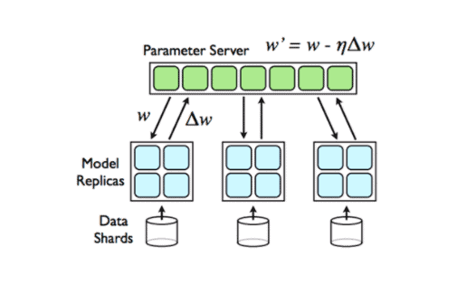
The diagram above shows the parameter server-based architecture. In this approach, computational nodes are partitioned into workers and parameter servers. Each worker “owns” a portion of the data and workload, and the parameter servers together maintain the globally shared parameters (Scaling Distributed Machine Learning with the Parameter Server). At the beginning of each iteration, the worker pulls a completed copy of model parameters and pushes the newly updated model back to the parameter servers at the end of the iteration. As for synchronous SGD, the parameter servers will then average the model parameters pushed by all workers, creating an updated ‘global’ model for the workers to pull at the beginning of the next iteration.
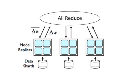
The MPI Allreduce method, on the other hand, doesn’t require a group of dedicated servers to store parameters. Instead, it makes use of the ring-allreduce (Bringing HPC techniques to deep learning) algorithm and the MPI (message passing interface) APIs to realize the model synchronization. For a model training cluster of N nodes, the model parameters will be split into N chunks, and each node participating in the ring-allreduce algorithm communicates with two of its peers 2∗(N−1) times. Thus, theoretically speaking, the model averaging time is only related to the size of the model, regardless of the number of nodes. During this communication, a node sends and receives chunks of the data buffer. In the first N−1 iterations, received values are added to the values in the node’s buffer. In the second N−1 iterations, received values replace the values held in the node’s buffer. The MPI APIs were developed by the high performance computing community to realize the model parameters synchronization, and Open MPI is one of the widely used MPI implementations that is developed and maintained by a consortium of academic, research, and industry partners.
As for the performance of the parameter server based method compared against the MPI Allreduce method, the benchmark results in both Uber and MXNet show that MPI Allreduce outperforms parameter server in small-scale number of nodes (8-64) (Horovod: fast and easy distributed deep learning in TensorFlow and Extend MXNet Distributed Training by MPI AllReduce).
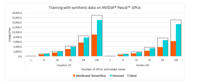
The figure above is the result of Uber’s benchmarks, parameter server (Tensorflow native) versus MPI Allreduce (Horovod), which compares the images processed per second with a standard distributed TensorFlow and Horovod when running a distributed training job over different numbers of NVIDIA Pascal GPUs for Inception V3 and ResNet-101 TensorFlow models over 25GbE TCP. Meanwhile, MXNet’s benchmark results below also show that even when the number of parameter servers and workers are all 8, the performance of the MPI Allreduce method is still higher than the parameter server approach.
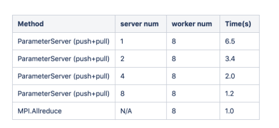
From the performance data, we can draw the following conclusions (Extend MXNet Distributed Training by MPI AllReduce): 1) the MPI Allreduce method doesn’t need an extra server node and can achieve better performance than the parameter server-based method can reach in synchronous SGD multi-node training. (In the parameter server-based approach, if not well configured, insufficient servers will be the hot spots in terms of network bandwidth.) 2) Moreover, the MPI Allreduce method is easier for hardware deployment. (In the parameter server-based approach, the configuration of server: worker ratio needs to be meticulously calculated and it’s not fixed (depending upon topology and network bandwidth).)
Traditionally, Tensorflow supports the parameter server-based approach, while PyTorch and Horovod support the MPI Allreduce method. However, starting from r1.3, Tensorflow is also starting to support the MPI Allreduce approach (with experimental support in r1.4).
Note. The parameter server-based approaches are capable of supporting both synchronous and asynchronous SGD, like Tensorflow. To the best of our knowledge, all of the current implementations of the MPI Allreduce method only support synchronous SGD.
With this fundamental knowledge, let’s move on to the programming part of distributed model training, with both the parameter server-based and the MPI Allreduce methods, and see how to use both in CML.
Programming with the parameter server-based approach in CML
(Full script here)
This section will present an overview of writing a parameter server-based distributed model training code in CML. We will use Tensorflow native distributed APIs and CML’s distributed API (cdsw.launch_worker) to demonstrate.
First, each parameter server or worker in the distributed Tensorflow is a Python process. So it is natural for us to use CML workers (or containers) to represent both TF parameter servers or TF workers and invoke these CML workers in the main CML session with the cdsw.launch_workers(…) function. In cdsw.launch_workers(…), we can also specify different Python program files for TF parameter servers and TF workers. Following that, the main CML session needs to collect the host names or IP addresses of each container and send them to all CML child workers, to create the cluster specification (tf.train.ClusterSpec). In CML, there are actually a number of methods to obtain the IP addresses of each child worker, and we are going to introduce a method using the new await_workers function, which is officially available in the CML Docker engine V10.
The await_workers function is used to wait for the startup of other CML containers specified by their session IDs. The return value of await_workers is a Python dictionary, with an item whose key name is ip_address, bringing with it their IP addresses. The code below shows how to use cdsw_await_workers in the CML main session. Please note that if some of the containers failed to start up after a specified amount of time (for example, 60 seconds for the following code), the return value of await_workers will bring an item with key name failures, containing the session IDs of failed workers.
# CML main session
import cdsw
workers = cdsw.launch_workers(NUM_WORKERS,
                              cpu=0.5, memory=2,
                              script=”...”)
worker_ids = [worker["id"] for worker in workers]
running_workers = cdsw.await_workers(worker_ids,
                              wait_for_completion=False,
                              timeout_seconds=60)
worker_ips = [worker["ip_address"] for worker in \
                              running_workers["workers"]]
After acquiring and distributing the IP addresses of all TF parameter servers and TF workers, every worker needs to construct the instances. In the code snippet below, PS1:PORT1 stands for the IP address and port number of the first TF parameter server process, PS2:PORT2 stands for the IP address and port number of the second TF parameter server process, while WORKER1:PORT1 for the IP address and port number of the first TF worker, etc.
cluster = tf.train.ClusterSpec({"ps": ["PS1:PORT1","PS2:PORT2",...],
                     "worker": ["WORKER1:PORT1","WORKER2:PORT2",...]})
server = tf.train.Server(cluster, job_name="PS or WORKER",
                                  task_index=NUM)
For a TF parameter server container, call server.join() to wait until all the other parameter server processes and worker processes join in the cluster.
server.join()
For a TF worker, all of the modeling and training code needs to be programmed. The modeling part is literally the same as the monolithic Tensorflow program if you are using data parallelism. The training code, however, has at least 2 distinct differences from the monolithic Tensorflow program.
- Wrap the model optimizer with tf.train.SyncReplicasOptimizer, which is the synchronous SGD version of a monolithic Tensorflow optimizer. Here is the sample code of tf.train.SyncReplicasOptimizer.
optimizer = tf.train.AdamOptimizer(learning_rate=...)
sr_optim = tf.train.SyncReplicasOptimizer(
                     optimizer,
                     replicas_to_aggregate=NUM_WORKER,
                     total_num_replicas=NUM_WORKER)
- Normally, it is recommended to use tf.train.MonitoredTrainingSession instead of tf.Session to do training, as MonitoredTrainingSession provides a lot of monitoring and automatic administrative functionalities that are essential for a productive distributed model training environment.
Note. tf.train.Supervisor has been deprecated in recent versions of Tensorflow, and it is now recommended to use tf.train.MonitoredTrainingSession in place of tf.train.Supervisor.
Repeating the programming procedure described above every time we write the distributed Tensorflow code is not only time-consuming but also error-prone. Thus we wrap them up in a function (cdsw_tensorflow_utils.run_cluster), released together with this blog post, so as to automate the whole procedure, so that data scientists only have to specify the number of parameter servers, workers, and the training code. The script containing the function can be found here. The following program demonstrates how to create a distributed Tensorflow cluster using cdsw_tensorflow_utils.run_cluster.
cluster_spec, session_addr = cdsw_tensorflow_utils.run_cluster(
                                 n_workers=n_workers,
                                 n_ps=n_ps,
                                 cpu=0.5,
                                 memory=2,
                                 worker_script="train.py")
The file train.py is where the model definition and training code resides, and it looks much like the monolithic Tensorflow code. The structure of train.py is as follows:.
import sys, time
import tensorflow as tf

# config model training parameters
batch_size = 100
learning_rate = 0.0005
training_epochs = 20

# load data set
from tensorflow.examples.tutorials.mnist import input_data
mnist = input_data.read_data_sets('MNIST_data', one_hot=True)

# Define the run() function with the following arguments
# And this function will be invoked within CML API
def run(cluster, server, task_index):

    # Specify cluster and device in tf.device() function
    with tf.device(tf.train.replica_device_setter(
        worker_device="/job:worker/task:%d" % task_index,
        cluster=cluster)):

        # Count the number of updates
        global_step = tf.get_variable(
            'global_step',
            [],
            initializer = tf.constant_initializer(0),
            trainable = False)

        # Model definition
        …

    # Define a tf.train.Supervisor instance
    # and use it to start model training
    sv = tf.train.Supervisor(is_chief=(task_index == 0),
                            global_step=global_step,
                            init_op=init_op)
    with sv.prepare_or_wait_for_session(server.target) as sess:

        # Model training code
        …

    # Stop the Supervisor instance
    sv.stop()
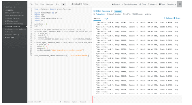
The screenshot below shows the execution process of a distributed model training program with asynchronous model averaging on CML, using the CML built-in API introduced above.
Preview of the MPI Allreduce approach to programming in CML
This section provides an overview of performing distributed model training with the MPI Allreduce method in CML, and uses Horovod to implement it.
When using Horovod, a driver node (the CML main session in this context) needs to perform SSH passwordless login to Horovod worker nodes to bring up all the model training processes. To enable SSH passwordless login for user cdsw in CML, two setting steps are required: 1) setting passwordless authentication for user cdsw, and 2) specifying the default SSH listening port from 22 to 2222.
- Enabling SSH passwordless authentication for user cdsw in CML is pretty easy. You only need to go to your user settings page and copy the public key from the ‘outbound ssh’ tab into the ‘remote editing’ tab. After that, all sessions within the same user are able to use passwordless login to ssh into each other.
Note: This step is not required in the April 14 and later versions of CML.
- The sshd listening port of the CML engine is 2222. When using the mpirun command to invoke Horovod workers, you can create a ~/.ssh/config file, and input like the following.
Host 100.66.0.29
Port 2222
Host 100.66.0.30
Port 2222
Otherwise, when using horovodrun command, you simply have to specify an extra argument of -p 2222 for horovodrun.
Next, launch several CML worker containers, and wait until obtaining the IP addresses of the launched workers. (This approach is exactly the same as the method used in the parameter server based method of distributed deep learning.) Then, start the Horovod model training processes in these launched workers, which can be implemented by invoking the horovodrun command in the os.system() Python function. These two steps can all be done with the Python code in the CML main session. Below is the sample code to implement the functionalities, and train.py is just Python code for model training.
# CML main session
Import os
import cdsw

workers = cdsw.launch_workers(NUM_WORKERS,
                              cpu=0.5, memory=2,
                              script=”...”)
worker_ids = [worker["id"] for worker in workers]
running_workers = cdsw.await_workers(worker_ids,
                              wait_for_completion=False,
                              timeout_seconds=60)
worker_ips = [worker["ip_address"] for worker in \
                              Running_workers["workers"]]
cmd="horovodrun -np {} -H {} -p 2222 python train.py".format(
                              len(worker_ips),
                              ",".join(worker_ips))

os.system(cmd)
In the MPI Allreduce approach, there is still a requirement to modify the model training file, i.e., train.py of sample code above. In train.py, there are 2 major modifications in the code: 1) creating the clustered environment among the worker processes, and 2) performing model averaging. We will address these topics in the next post of this series, in addition to taking a technical deep dive into the MPI Allreduce approach and its implementation in CML, and presenting the performance benchmark results of these methods.
Get more details about CML direct from technical experts by watching this How-To video series.
Editor's Choice