Image Classification using Convolutional Neural Network with Python
This article was published as a part of the Data Science Blogathon
Introduction:
Hello guys! In this blog, I am going to discuss everything about image classification.
In the past few years, Deep Learning has been proved that its a very powerful tool due to its ability to handle huge amounts of data. The use of hidden layers exceeds traditional techniques, especially for pattern recognition. One of the most popular Deep Neural Networks is Convolutional Neural Networks(CNN).
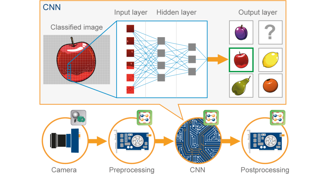
A convolutional neural network(CNN) is a type of Artificial Neural Network(ANN) used in image recognition and processing which is specially designed for processing data(pixels).
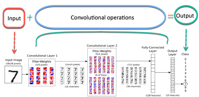
Image Source: Google.com
Before moving further we need to understand what is the neural network? Let’s go…
Neural Network:
A neural network is constructed from several interconnected nodes called “neurons”. Neurons are arranged into the input layer, hidden layer, and output layer. The input layer corresponds to our predictors/features and the Output layer to our response variable/s.
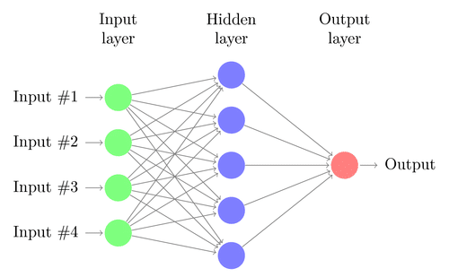
Image Source: Google.com
Multi-Layer Perceptron(MLP):
The neural network with an input layer, one or more hidden layers, and one output layer is called a multi-layer perceptron (MLP). MLP is Invented by Frank Rosenblatt in the year of 1957. MLP given below has 5 input nodes, 5 hidden nodes with two hidden layers, and one output node
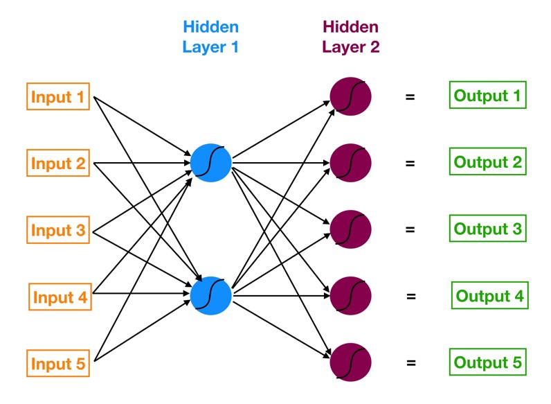
Image Source: Google.com
How does this Neural Network work?
– Input layer neurons receive incoming information from the data which they process and distribute to the hidden layers.
– That information, in turn, is processed by hidden layers and is passed to the output neurons.
– The information in this artificial neural network(ANN) is processed in terms of one activation function. This function actually imitates the brain neurons.
– Each neuron contains a value of activation functions and a threshold value.
– The threshold value is the minimum value that must be possessed by the input so that it can be activated.
– The task of the neuron is to perform a weighted sum of all the input signals and apply the activation function on the sum before passing it to the next(hidden or output) layer.
Let us understand what is weightage sum?
Say that, we have values 𝑎1, 𝑎2, 𝑎3, 𝑎4 for input and weights as 𝑤1, 𝑤2, 𝑤3, 𝑤4 as the input to one of the hidden layer neuron say 𝑛𝑗, then the weighted sum is represented as
𝑆𝑗 = σ 𝑖=1to4 𝑤𝑖*𝑎𝑖 + 𝑏𝑗
where 𝑏𝑗 : bias due to node
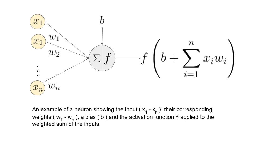
Image Source: Google.com
What are the Activation Functions?
These functions are needed to introduce a non-linearity into the network. The activation function is applied and that output is passed to the next layer.
*Possible Functions*
• Sigmoid: Sigmoid function is differentiable. It produces output between 0 and 1.
• Hyperbolic Tangent: Hyperbolic Tangent is also differentiable. This Produces output between -1 and 1.
• ReLU: ReLU is Most popular function. ReLU is used widely in deep learning.
• Softmax: The softmax function is used for multi-class classification problems. It is a generalization of the sigmoid function. It also produces output between 0 and 1
Now, let’s go with our topic CNN…
CNN:
Now imagine there is an image of a bird, and you want to identify it whether it is really a bird or something other. The first thing you should do is feed the pixels of the image in the form of arrays to the input layer of the neural network (MLP networks used to classify such things). The hidden layers carry Feature Extraction by performing various calculations and operations. There are multiple hidden layers like the convolution, the ReLU, and the pooling layer that performs feature extraction from your image. So finally, there is a fully connected layer that you can see which identifies the exact object in the image. You can understand very easily from the following figure:
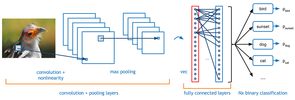
Image Source: Google.com
Convolution:-
Convolution Operation involves matrix arithmetic operations and every image is represented in the form of an array of values(pixels).
Let us understand example:
a = [2,5,8,4,7,9]
b = [1,2,3]
In Convolution Operation, the arrays are multiplied one by one element-wise, and the product is grouped or summed to create a new array that represents a*b.
The first three elements of matrix a are now multiplied by the elements of matrix b. The product is summed to get the result and stored in a new array of a*b.
This process remains continuous until the operation gets completed.
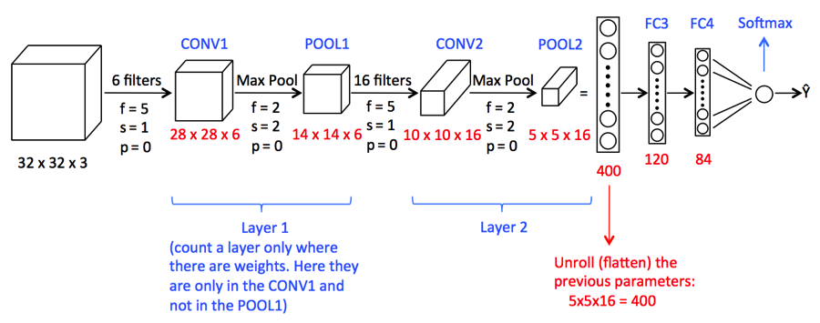
Image Source: Google.com
Pooling:
After the convolution, there is another operation called pooling. So, in the chain, convolution and pooling are applied sequentially on the data in the interest of extracting some features from the data. After the sequential convolutional and pooling layers, the data is flattened
into a feed-forward neural network which is also called a Multi-Layer Perceptron.
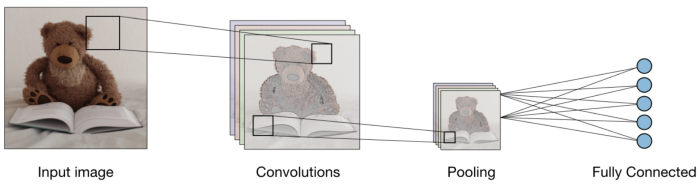
Image Source: Google.com
Up to this point, we have seen concepts that are important for our building CNN model.
Now we will move forward to see a case study of CNN.
1) Here we are going to import the necessary libraries which are required for performing CNN tasks.
import NumPy as np
%matplotlib inline
import matplotlib.image as mpimg
import matplotlib.pyplot as plt
import TensorFlow as tf
tf.compat.v1.set_random_seed(2019)
2) Here we required the following code to form the CNN model
model = tf.keras.models.Sequential([
    tf.keras.layers.Conv2D(16,(3,3),activation = "relu" , input_shape = (180,180,3)) ,
    tf.keras.layers.MaxPooling2D(2,2),
    tf.keras.layers.Conv2D(32,(3,3),activation = "relu") ,
    tf.keras.layers.MaxPooling2D(2,2),
    tf.keras.layers.Conv2D(64,(3,3),activation = "relu") ,
    tf.keras.layers.MaxPooling2D(2,2),
    tf.keras.layers.Conv2D(128,(3,3),activation = "relu"),
    tf.keras.layers.MaxPooling2D(2,2),
    tf.keras.layers.Flatten(),
    tf.keras.layers.Dense(550,activation="relu"),      #Adding the Hidden layer
    tf.keras.layers.Dropout(0.1,seed = 2019),
    tf.keras.layers.Dense(400,activation ="relu"),
    tf.keras.layers.Dropout(0.3,seed = 2019),
    tf.keras.layers.Dense(300,activation="relu"),
    tf.keras.layers.Dropout(0.4,seed = 2019),
    tf.keras.layers.Dense(200,activation ="relu"),
    tf.keras.layers.Dropout(0.2,seed = 2019),
    tf.keras.layers.Dense(5,activation = "softmax")   #Adding the Output Layer
])
A convoluted image can be too large and so it is reduced without losing features or patterns, so pooling is done.
Flatten()- Flattening transforms a two-dimensional matrix of features into a vector of features.
3) Now let’s see a summary of the CNN model
model.summary()
It will print the following output
Model: "sequential"
_________________________________________________________________
Layer (type)                 Output Shape              Param #
=================================================================
conv2d (Conv2D)              (None, 178, 178, 16)      448
_________________________________________________________________
max_pooling2d (MaxPooling2D) (None, 89, 89, 16)        0
_________________________________________________________________
conv2d_1 (Conv2D)            (None, 87, 87, 32)        4640
_________________________________________________________________
max_pooling2d_1 (MaxPooling2 (None, 43, 43, 32)        0
_________________________________________________________________
conv2d_2 (Conv2D)            (None, 41, 41, 64)        18496
_________________________________________________________________
max_pooling2d_2 (MaxPooling2 (None, 20, 20, 64)        0
_________________________________________________________________
conv2d_3 (Conv2D)            (None, 18, 18, 128)       73856
_________________________________________________________________
max_pooling2d_3 (MaxPooling2 (None, 9, 9, 128)         0
_________________________________________________________________
flatten (Flatten)            (None, 10368)             0
_________________________________________________________________
dense (Dense)                (None, 550)               5702950
_________________________________________________________________
dropout (Dropout)            (None, 550)               0
_________________________________________________________________
dense_1 (Dense)              (None, 400)               220400
_________________________________________________________________
dropout_1 (Dropout)          (None, 400)               0
_________________________________________________________________
dense_2 (Dense)              (None, 300)               120300
_________________________________________________________________
dropout_2 (Dropout)          (None, 300)               0
_________________________________________________________________
dense_3 (Dense)              (None, 200)               60200
_________________________________________________________________
dropout_3 (Dropout)          (None, 200)               0
_________________________________________________________________
dense_4 (Dense)              (None, 5)                 1005
=================================================================
Total params: 6,202,295
Trainable params: 6,202,295
Non-trainable params: 0
4) So now we are required to specify optimizers.
from tensorflow.keras.optimizers import RMSprop,SGD,Adam
adam=Adam(lr=0.001)
model.compile(optimizer='adam', loss='categorical_crossentropy', metrics = ['acc'])
Optimizer is used to reduce the cost calculated by cross-entropy
The loss function is used to calculate the error
The metrics term is used to represent the efficiency of the model
5)In this step, we will see how to set the data directory and generate image data.
bs=30         #Setting batch size
train_dir = "D:/Data Science/Image Datasets/FastFood/train/"   #Setting training directory
validation_dir = "D:/Data Science/Image Datasets/FastFood/test/"   #Setting testing directory
from tensorflow.keras.preprocessing.image import ImageDataGenerator
# All images will be rescaled by 1./255.
train_datagen = ImageDataGenerator( rescale = 1.0/255. )
test_datagen  = ImageDataGenerator( rescale = 1.0/255. )
# Flow training images in batches of 20 using train_datagen generator
#Flow_from_directory function lets the classifier directly identify the labels from the name of the directories the image lies in
train_generator=train_datagen.flow_from_directory(train_dir,batch_size=bs,class_mode='categorical',target_size=(180,180))
# Flow validation images in batches of 20 using test_datagen generator
validation_generator =  test_datagen.flow_from_directory(validation_dir,
                                                         batch_size=bs,
                                                         class_mode  = 'categorical',
                                                         target_size=(180,180))
The output will be:
Found 1465 images belonging to 5 classes.
Found 893 images belonging to 5 classes.
6) Final step of the fitting model.
history = model.fit(train_generator,
                    validation_data=validation_generator,
                    steps_per_epoch=150 // bs,
                    epochs=30,
                    validation_steps=50 // bs,
                    verbose=2)
The output will be:
Epoch 1/30
5/5 - 4s - loss: 0.8625 - acc: 0.6933 - val_loss: 1.1741 - val_acc: 0.5000
Epoch 2/30
5/5 - 3s - loss: 0.7539 - acc: 0.7467 - val_loss: 1.2036 - val_acc: 0.5333
Epoch 3/30
5/5 - 3s - loss: 0.7829 - acc: 0.7400 - val_loss: 1.2483 - val_acc: 0.5667
Epoch 4/30
5/5 - 3s - loss: 0.6823 - acc: 0.7867 - val_loss: 1.3290 - val_acc: 0.4333
Epoch 5/30
5/5 - 3s - loss: 0.6892 - acc: 0.7800 - val_loss: 1.6482 - val_acc: 0.4333
Epoch 6/30
5/5 - 3s - loss: 0.7903 - acc: 0.7467 - val_loss: 1.0440 - val_acc: 0.6333
Epoch 7/30
5/5 - 3s - loss: 0.5731 - acc: 0.8267 - val_loss: 1.5226 - val_acc: 0.5000
Epoch 8/30
5/5 - 3s - loss: 0.5949 - acc: 0.8333 - val_loss: 0.9984 - val_acc: 0.6667
Epoch 9/30
5/5 - 3s - loss: 0.6162 - acc: 0.8069 - val_loss: 1.1490 - val_acc: 0.5667
Epoch 10/30
5/5 - 3s - loss: 0.7509 - acc: 0.7600 - val_loss: 1.3168 - val_acc: 0.5000
Epoch 11/30
5/5 - 4s - loss: 0.6180 - acc: 0.7862 - val_loss: 1.1918 - val_acc: 0.7000
Epoch 12/30
5/5 - 3s - loss: 0.4936 - acc: 0.8467 - val_loss: 1.0488 - val_acc: 0.6333
Epoch 13/30
5/5 - 3s - loss: 0.4290 - acc: 0.8400 - val_loss: 0.9400 - val_acc: 0.6667
Epoch 14/30
5/5 - 3s - loss: 0.4205 - acc: 0.8533 - val_loss: 1.0716 - val_acc: 0.7000
Epoch 15/30
5/5 - 4s - loss: 0.5750 - acc: 0.8067 - val_loss: 1.2055 - val_acc: 0.6000
Epoch 16/30
5/5 - 4s - loss: 0.4080 - acc: 0.8533 - val_loss: 1.5014 - val_acc: 0.6667
Epoch 17/30
5/5 - 3s - loss: 0.3686 - acc: 0.8467 - val_loss: 1.0441 - val_acc: 0.5667
Epoch 18/30
5/5 - 3s - loss: 0.5474 - acc: 0.8067 - val_loss: 0.9662 - val_acc: 0.7333
Epoch 19/30
5/5 - 3s - loss: 0.5646 - acc: 0.8138 - val_loss: 0.9151 - val_acc: 0.7000
Epoch 20/30
5/5 - 4s - loss: 0.3579 - acc: 0.8800 - val_loss: 1.4184 - val_acc: 0.5667
Epoch 21/30
5/5 - 3s - loss: 0.3714 - acc: 0.8800 - val_loss: 2.0762 - val_acc: 0.6333
Epoch 22/30
5/5 - 3s - loss: 0.3654 - acc: 0.8933 - val_loss: 1.8273 - val_acc: 0.5667
Epoch 23/30
5/5 - 3s - loss: 0.3845 - acc: 0.8933 - val_loss: 1.0199 - val_acc: 0.7333
Epoch 24/30
5/5 - 3s - loss: 0.3356 - acc: 0.9000 - val_loss: 0.5168 - val_acc: 0.8333
Epoch 25/30
5/5 - 3s - loss: 0.3612 - acc: 0.8667 - val_loss: 1.7924 - val_acc: 0.5667
Epoch 26/30
5/5 - 3s - loss: 0.3075 - acc: 0.8867 - val_loss: 1.0720 - val_acc: 0.6667
Epoch 27/30
5/5 - 3s - loss: 0.2820 - acc: 0.9400 - val_loss: 2.2798 - val_acc: 0.5667
Epoch 28/30
5/5 - 3s - loss: 0.3606 - acc: 0.8621 - val_loss: 1.2423 - val_acc: 0.8000
Epoch 29/30
5/5 - 3s - loss: 0.2630 - acc: 0.9000 - val_loss: 1.4235 - val_acc: 0.6333
Epoch 30/30
5/5 - 3s - loss: 0.3790 - acc: 0.9000 - val_loss: 0.6173 - val_acc: 0.8000
The above function trains the neural network using the training set and evaluates its performance on the test set. The functions return two metrics for each epoch ‘acc’ and ‘val_acc’ which are the accuracy of predictions obtained in the training set and accuracy attained in the test set respectively.
Conclusion:
Hence, we see that sufficient accuracy has been met. However, anyone can run this model by increasing the number of epochs or any other parameters.
I hope you liked my article. Do share with your friends, colleagues.
The media shown in this article are not owned by Analytics Vidhya and are used at the Author’s discretion.
I am data science enthusiastic, tech savvy and traveller.


Very nice information 😉
Ca you share the dataset that you used.