Machine Learning 101: The What, Why, and How of Weighting

Weighting is a technique for improving models. In this article, learn more about what weighting is, why you should (and shouldn’t) use it, and how to choose optimal weights to minimize business costs.

comments

By Eric Hart, Altair.

Introduction

One thing I get asked about a lot is weighting. What is it? How do I do it? What do I need to worry about? By popular demand, I recently put together a lunch-and-learn at my company to help address all these questions. The goal was to be applicable to a large audience, (e.g., with a gentle introduction), but also some good technical advice/details to help practitioners. This blog was adapted from that presentation.

Model Basics

Before we talk about weighting, we should all get on the same page about what a model is, what they are used for, and some of the common issues that modelers run into. Models are basically tools that humans can use to (over-)simplify the real world in a rigorous way. Often, they take the form of equations or rules sets, and they usually try to capture patterns that are found in data. People often divide models into one of two high-level categories in terms of what they are being used for (and yes, there can be overlap): Inference and Prediction. Inference means trying to use models to help understand the world. Think scientists trying to uncover physical truths from data. Prediction means trying to make guesses about what is going to happen. For most of the rest of this discussion, we’re going to be focused on models built with purposes of prediction in mind.

If you’re building a model to make predictions, you’re going to need a way to measure how good that model is at making predictions. A good place to start is with Accuracy. The Accuracy of a model is simply the percentage of its predictions, which turn out to be correct. This can be a useful measure, and indeed it’s essentially the default measure for a lot of automatic tools for training models, but it certainly has some shortcomings. For one thing, accuracy doesn’t care about how likely the model thinks each prediction is (the probabilities associated with the guesses). Accuracy also doesn’t care about which predictions the model makes (e.g. if it’s deciding between a positive or negative event, accuracy doesn’t give one of them priority over the other). Accuracy also doesn’t care about differences between the set of records the accuracy is measured on and the real population which the model is supposed to apply to. These things can be important.

Let’s jump into an example. Recently, the 2019 World Series concluded. I’m going to contrast some predictions for that world series below. Spoiler Alert: I’m going to tell you who won the world series.

The 2019 world series took place between the Washington Nationals and the Houston Astros

Let’s investigate some models. I have an internal model in my head, which I won’t explain. It gave these predictions for each of the 7 games of the series:

Apparently, I was pretty high on the Nationals. Meanwhile, one of my favourite websites, FiveThirtyEight, has an advanced statistical model which they use to predict games. It gave these predictions:

It’s worth noting: these are individual game predictions, made in advance of each game if it was going to happen; these are not predictions for the series as a whole. Since the series is a best-of-seven, once a team wins 4 games, no more games will be played, so obviously neither of the two sets of predictions above will happen exactly as is.

These predictions are based on things like team strength, home field advantage, and specifics of which pitcher is starting each game. FiveThirtyEight’s model predicted the home team to win in every game, except game 5, when Houston’s best pitcher, Gerrit Cole, was pitching in Washington.

Anyway, let’s spoil the series, see what happened, and compare accuracy. Here was the real result:

The series went 7 games, with Washington winning the first and last 2. (As an aside, the away team won every game in this series, which had never happened before in this, or any other, major North American professional sport.)

So, let’s look at how we each did:

My result:

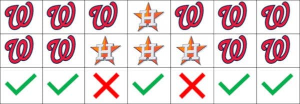
I got 5 of the 7 games right, for an accuracy of 0.71

FiveThirtyEight’s Result:

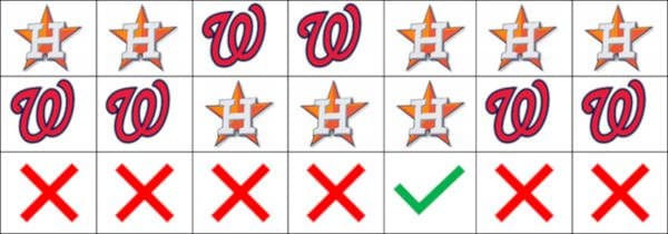
FiveThirtyEight got only 1 game right, for an accuracy of 0.14.

So, you might be tempted to think that my model is better than FiveThirtyEight’s, or at least that it did better in this case. But predictions aren’t the whole story. FiveThirtyEight’s model comes not only with predictions, but with helpful probabilities, suggesting how likely FiveThirtyEight thinks each team is to win. In this case, those probabilities looked like this:

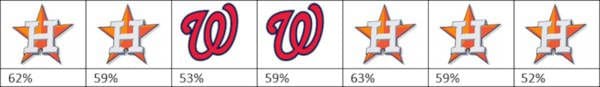
Meanwhile, I’m the jerk who is always certain he’s right about everything. You all know the type. My probabilities looked like this.

With this in mind, even though I had a higher accuracy, you might rethink which model you prefer.

It’s important to discuss this because we’re going to be talking about accuracy again soon while addressing some of the shortcomings of certain models. It’s important to remember that accuracy can be a useful metric, but it doesn’t always give you a full picture. There are other tools for measuring the quality of models that pay attention to things like probabilities, and other more subtle concepts than just prediction. A few examples I like to use are Lift Charts, ROC Curves, and Precision-Recall Curves. These are good tools that can be used to help choose a good model, but none of them are fool-proof on their own. Also, these tools are more visual, and often, machine learning algorithms need a single number underneath, so accuracy ends up getting baked into a lot of algorithms as the default measure of choice, even when that’s detrimental to some external goal.

The What of Weighting

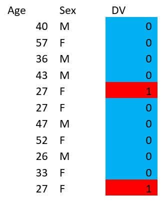
Consider the following data table:

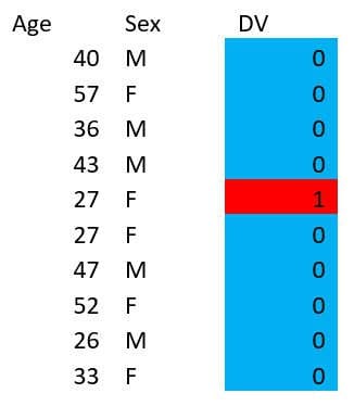
Say you want to build a model to predict the value of ‘DV’ using only Age and Sex. Because there is only one example with DV=1, you may have a hard time predicting that value. If this is a dataset about credit lending, and the DV is whether someone is going to default (1 meaning they defaulted), you may care more about being correct on the DV=1 cases than the DV=0 cases. Take a minute and see if you can come up with a good model (e.g. some rules) to predict DV=1 on this dataset. (Spoiler, you can’t possibly get 100% accuracy).

Here are some possible examples:

Intercept Only Model
- Always Predict 0
- Accuracy = 0.9
27 Year Olds
- Predict DV=1 for 27-year-olds, and 0 otherwise
- Accuracy = 0.9
Young Women
- Predict DV=1 for women under 30, and 0 otherwise
- Accuracy = 0.9

All these models have the same accuracy, but some of them may be more useful in certain use cases. If you ask a decision tree or a logistic regression algorithm to build a model on these datasets, they will both give you model #1 by default. The models don’t know that you might care more about the DV=1 cases. So, how can we make the DV=1 cases more important to the model?

Idea #1: Oversampling: Duplicate existing rare event records and leave common event records alone.

Idea #2: Undersampling: Remove some of the common event records, keep all the rare event records.

In both cases, we manually use a different population to train the model on than what we naturally had, with the express purpose of affecting the model we’re going to build.

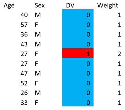
Weighting is kind of like this, but instead of duplicating or removing records, we assign different weights to each record as a separate column. For example, instead of doing this:

We could just do this:

You might legitimately ask if it’s possible for machine learning algorithms to handle weighted data this way, but a legitimate answer is: “yes, it’s fine, don’t worry about it.”

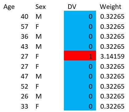
In fact, we don’t even need to give integer weights. You could even do something like this:

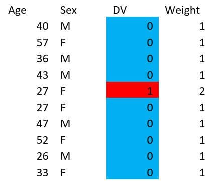
But for now, let’s stick to the integer weights. Say you want to build your model on the weighted dataset above:

Then if we revisit the possible models we discussed before, we see this:

Intercept Only Model
- Weighted Accuracy (for training model): 0.82
- Real Accuracy = 0.9
27 Year Olds
- Weighted Accuracy (for training model): 0.91
- Real Accuracy = 0.9
Young Women
- Weighted Accuracy (for training model): 0.91
- Real Accuracy = 0.9

By weighting, even though we haven’t changed the real accuracy, we’ve changed the weighted accuracy, which would cause the first option to be less desirable than the latter two at training time. In fact, if you build a model on this weighted table, a decision tree naturally finds the second model, while a Logistic Regression naturally finds the third model.

A common question I get about weighting is: how do you handle things after model training? Do you have to apply your weights during validation or deployment? The answer is No! The point of weighting was to influence your model, not to influence the world. Once your model is trained, your weights are no longer needed (or useful) for anything.

The Why of Weighting

In the previous section we got a vague sense of why you might want to use weighting to influence model selection, but let’s dive in a little deeper.

One reason you might want to use weighting is if your training data isn’t a representative sample of the data you plan to apply your model to. Pollsters come across this problem all the time. Fun fact: with a truly random sample of just 2500 people, pollsters could predict election results within +/- 1%. The problem is how to get a truly random sample. This is difficult, so pollsters routinely apply weights to different poll participants to get the sample demographics to more closely match the expected voting demographics. There’s a great story from 2016 about how one person was responsible for strongly skewing an entire poll. You can read about it here.

Here’s a common argument I hear for another reason you might want to use weighting:

Fraud is rare
Need to upweight rare cases
Then the model performs better overall

This common argument turns out to be wrong. In general, weighting causes models to perform worse overall but causes them to perform better on certain segments of the population. In the case of fraud, the missing piece from the above argument is that failing to catch fraud is usually more expensive than falsely flagging non-fraudulent transactions.

What we really want to talk about as a good reason for weighting is cost-sensitive classification. Some examples:

In fraud detection, false negatives tend to cost more than false positives
In credit lending, defaults tend to be more expensive than rejected loans that would not have defaulted
In preventative maintenance, part failures tend to be more expensive than premature maintenance

All of these are only true within reason. You can’t go all the way to the extreme, because flagging every transaction as fraudulent, rejecting all loan applications, or spending all your time repairing systems instead of using them are all clearly bad business decisions. But the point is, certain kinds of misclassification are more expensive than other kinds of misclassification, so we might want to influence our model to make decisions that are wrong more often, but still less expensive overall. Using weighting is a reasonable tool to help solve this problem.

The How of Weighting

Note upfront: a lot of the great information from this section comes from the same paper.

This brings us to an important question: how do you weight? With most modern data science software, you just use computer magic and the weights are taken care of for you.

But, of course, there are still important decisions to make. Should you over-sample or under-sample, or just use weighting? Should you use advanced packages like SMOTE or ROSE? What weights should you pick?

Well, good news: I’m going to tell you the optimal thing to do. But of course, since I’m a data scientist, I’m going to give you a lot of caveats first:

This method is only “optimal” for cost-sensitive classification issues (e.g. you have different costs for different outcomes of what you’re predicting). I’m not going to help pollsters out here (sorry).
This method assumes you know the costs associated with your problem, and that the costs are fixed. If the true costs are unknown, or variable, this gets a lot harder.

Before we get right down to the formulas, let’s talk about a little trap that you might fall into baseline/reference errors. Here’s a typical looking cost-matrix example from the German credit dataset from the Statlog project.

	Actual Bad	Actual Good
Predict Bad	0	1
Predict Good	5	0

If you look at this for a few minutes, the rationale for where this came from becomes clear. This is meant to imply that if you misclassify someone who will default and give them a loan, you’ll lose $5, but if you misclassify someone who would not have defaulted and don’t give them credit, you lose the opportunity to make $1, which is itself a cost.

But something is wrong here. If the intention is that when you predict bad you don’t extend someone's credit, then it seems clear that the costs associated with predicting bad should be the same no matter what would have actually happened. In fact, this cost matrix is likely supposed to be this:

	Actual Bad	Actual Good
Predict Bad	0	0
Predict Good	5	-1

Where there is a negative cost (or benefit) of predicting good on someone who will actually repay their loan. While these two cost matrices are similar, they are not interchangeable. If you imagine a situation where you get one customer of each type, the first matrix suggests your total costs will be $6, and the second suggests your total costs will be $4. The second is clearly what is intended here. For this reason, it’s often beneficial to frame your matrix in terms of benefits instead of costs. That said, I’m still going to give the formula in terms of costs, and leave it to the reader to figure out how to translate it to a benefit formula.

So, say you have a cost matrix that looks like this:

	Actual Negative	Actual Positive
Predict Negative	C₀₀	C₀₁
Predict Positive	C₁₀	C₁₁

First, we will state 2 reasonableness criteria:

C₁₀ > C₀₀
C₀₁ > C₁₁

These criteria basically say that your costs are higher if you misclassify something than if you don’t. Reasonable, right?

Now define:

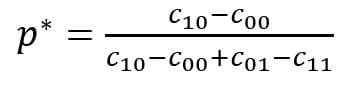
Then you should upweight your negative examples by (and leave your positive examples alone).

Actually, we can even take this a step further. Many machine learning models produce probabilities (as opposed to just predictions) and then use a threshold to convert that probability into a prediction. In other words, you have some rules like: if the probability of being positive is greater than 0.5 predict positive, otherwise predict negative. But you could instead have a rule that says something else, e.g., if the probability of being positive is greater than 0.75 predict positive, otherwise predict negative. The number here (0.5 or 0.75 in the above examples) is called a “threshold.” More on that is coming a little later, but for now, we can write down a formula for how to make a model with threshold p₀ act as though it has threshold p^*, we can do that by upweighting the negative examples by:

Note that in the special case where p₀ is 0.5 (as is typical), this reduces to the previous formula.

Once again, it’s worth noting that the case of variable costs is a lot harder. If you’re using decision trees, some smoothing is a good idea, but in general, it’s too involved to say much more here. But you can check out this paper for some ideas.

The Why Not of Weighting

Weighting is kind of like pretending to live in a fantasy world to make better decisions about the real world. Instead of this, you could just make better decisions without the pretend part.

Let’s return to our discussion about thresholds from the previous section. Instead of using weights to make a machine learning model with one threshold behave as though it had a different threshold, you could just change the threshold of that model directly. This would (presumably) lead to a poorly calibrated model, but it might still be a good business decision because it might reduce costs.

In fact, if you return to the cost matrix considered previously,

	Actual Negative	Actual Positive
Predict Negative	C₀₀	C₀₁
Predict Positive	C₁₀	C₁₁

the optimal threshold for making decisions in order to minimize costs is precisely p^*

This is often simpler, and empirical evidence suggests that adjusting the threshold directly works a little better than weighting in practice.

So basically, after all that talk about weighting, my general advice is, if possible don’t weight at all, but adjust your threshold instead! But of course, many of the ideas overlap, so hopefully, this discussion was still useful.

Also, one last tip: If you aren’t worried about cost-sensitive classification problems (e.g., problems where you have different costs associated with different predictions and DV cases), you probably shouldn’t be thinking about using weighting as a tool. Unless you’re a pollster.

Bio: Dr. Eric Hart is a Senior Data Scientist on the services team at Altair. He has a background in engineering and mathematics, and likes using his problem solving skill to tackle interesting data challenges. He’s also a Blokus world champion.

Related: