Before we understand more about Logistic Regression, let's first recap some important definitions which will give us a better understanding of the topic.
 
Logistic Regression comes under Supervised Learning. Supervised Learning is when the algorithm learns on a labeled dataset and analyses the training data. These labeled data sets have inputs and expected outputs.

Supervised learning can be further split into classification and regression.

 
Classification is about predicting a label, by identifying which category an object belongs to based on different parameters.

 
Regression is about predicting a continuous output, by finding the correlations between dependent and independent variables.

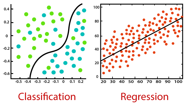
Source: Javatpoint

What is Logistic Regression?

 
Logistic Regression is a statistical approach and a Machine Learning algorithm that is used for classification problems and is based on the concept of probability. It is used when the dependent variable (target) is categorical.

It is widely used when the classification problem at hand is binary; true or false, yes or no, etc. For example, it can be used to predict whether an email is spam (1) or not (0).

Logistics regression uses the sigmoid function to return the probability of a label.

Sigmoid Function

 
Sigmoid Function is a mathematical function used to map the predicted values to probabilities. The function has the ability to map any real value into another value within a range of 0 and 1.

 
Code:

def sigmoid(z):
  return 1.0 / (1 + np.exp(-z))

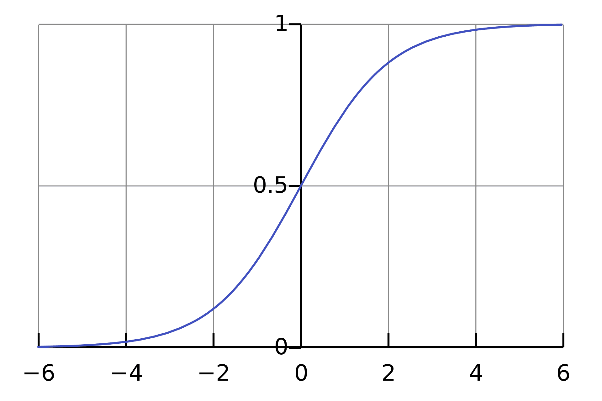
Source: Wikipedia

The rule is that the value of the logistic regression must be between 0 and 1. Due to the limitations of it not being able to go beyond the value 1, on a graph it forms a curve in the form of an "S". This is an easy way to identify the Sigmoid function or the logistic function.
In regards to Logistic Regression, the concept used is the threshold value. The threshold values help to define the probability of either 0 or 1. For example, values above the threshold value tend to 1, and a value below the threshold value tends to 0.

Type of Logistic Regression

1. Binomial: This means that there can be only two possible types of the dependent variables, such as 0 or 1, Yes or No, etc.
2. Multinomial: This means that there can be 3 or more possible unordered types of the dependent variable, such as "cat", "dogs", or "sheep"
3. Ordinal: This means that there can be 3 or more possible ordered types of dependent variables, such as "low", "Medium", or "High".

Linear and Logistic Regression

 
Linear Regression is similar to Logistic Regression but different.

Linear Regression assumes that there is a linear relationship between dependent and independent variables. It uses the line of best fit that describes two or more variables. The aim of Linear Regression is to accurately predict the output for the continuous dependent variable.

However, Logistic regression predicts the probability of an event or class that is dependent on other factors, therefore the output of Logistic Regression always lies between 0 and 1.

To find out more about the difference between Linear and Logistic Regression, you can read more about it on this link.

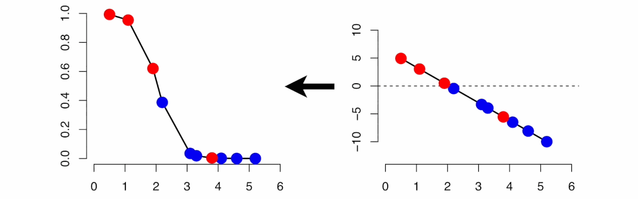
Source: gfycat

Cost Function

 
A Cost Function is a mathematical formula used to calculate the error, it is a difference between our predicted value and the actual value. It simply measures how wrong the model is in terms of its ability to estimate the relationship between x and y.

The value of the Cost Function can also be referred to as cost, loss, or error. Within Logistic Regression, the Cost Function we use is called Cross-Entropy, also known as Log Loss. The formula for this is:

If you would like to know more about different types of Cost Functions, click on this link.

Gradient Descent

 
In order to minimize our cost, we use Gradient Descent which estimates the parameters or weights of our model.

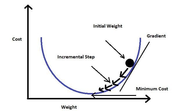Source: analyticsvidhya

Implementation of Logistic Regression

 
To give a simple example of how to implement Logistic Regression, I will use a dataset from kaggle which explores information about a product being purchased through an advertisement on social media.
Source of Dataset - https://www.kaggle.com/rakeshrau/social-network-ads

1. Load the dataset and libraries

# Import Libraries
import numpy as np
import pandas as pd
import matplotlib.pyplot as plt
from sklearn.model_selection import train_test_split
from math import exp
plt.rcParams["figure.figsize"] = (10, 6)# Download your chosen dataset
# Source of dataset - https://www.kaggle.com/rakeshrau/social-network-ads
# !wget "https://drive.google.com/uc?id=15WAD9_4CpUK6EWmgWVXU8YMnyYLKQvW8&export=download" -O data.csv -q# Load the dataset
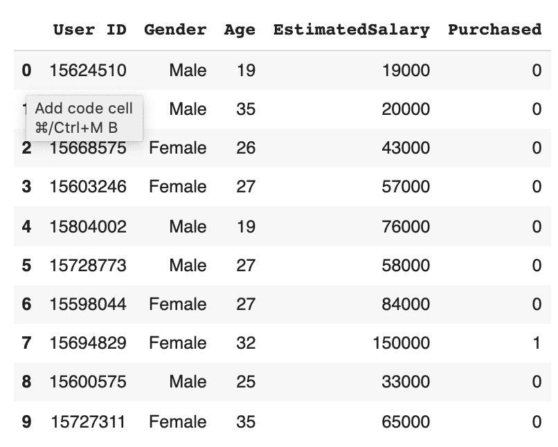
data = pd.read_csv("data.csv")
data.head(10)

2. Train/Test the Data

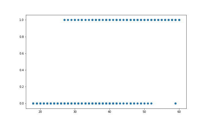
# Visualizing the dataset by Age and Purchased
plt.scatter(data['Age'], data['Purchased'])
plt.show()# Divide the Data into training set and test set
X_train, X_test, y_train, y_test = train_test_split(data['Age'], data['Purchased'], test_size=0.20)

3. Building the Model

 
We will need to normalise the data as well as shifting the mean to the origin. This is due to wanting to get accurate results because of the nature of the Logistic Equation.
We then create a method that will help us make predictions, which will return a probability. We can then move onto training the model. The model is trained for 300 epochs and The partial derivatives are calculated at each of these 300 epochs and the weights are updated.

# Building the Logistic Regression model

# Normalising the data
def normalize(X):
  return X - X.mean()

# Make predictions
def predict(X, b0, b1):
  return np.array([1 / (1 + exp(-1*b0 + -1*b1*x)) for x in X])

# The model
def logistic_regression(X, Y):

   X = normalize(X)

   # Initializing variables
   b0 = 0
   b1 = 0
   L = 0.001
   epochs = 300

   for epoch in range(epochs):
      y_pred = predict(X, b0, b1)
      D_b0 = -2 * sum((Y - y_pred) * y_pred * (1 - y_pred)) # Loss wrt b0
      D_b1 = -2 * sum(X * (Y - y_pred) * y_pred * (1 - y_pred)) # Loss wrt b1
      # Update b0 and b1
      b0 = b0 - L * D_b0
      b1 = b1 - L * D_b1

      return b0, b1

4. Training the Model

 
As mentioned above, the prediction equation will return a probability. Because this is a classification task, we will need to convert it into a binary value. In order to do this, we need to select a threshold. In this example, we will select the threshold 0.5 which means all the predicted values above 0.5 will be treated as 1 and everything below 0.5 will be treated as 0.

You can also calculate the accuracy by checking how many correct predictions we made and dividing it by the total number of test cases.

# Training the Model
b0, b1 = logistic_regression(X_train, y_train)# Making predictions and setting a thresholdX_test_norm = normalize(X_test)
y_pred = predict(X_test_norm, b0, b1)
y_pred = [1 if p >= 0.5 else 0 for p in y_pred]
# Plotting the data
plt.scatter(X_test, y_test)
plt.scatter(X_test, y_pred, c="red")
plt.show()# Calculating the accuracy
accuracy = 0
for i in range(len(y_pred)):
if y_pred[i] == y_test.iloc[i]:
accuracy += 1
print(f"Accuracy = {accuracy / len(y_pred)}")

Plot and Accuracy:

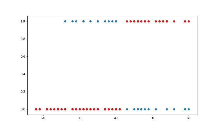
Accuracy = 0.85

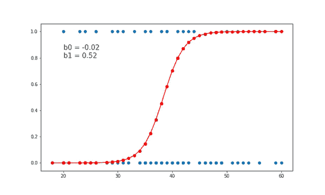
Using this below gify helps us to visually see how the value of weights b0 and b1 are updated at each iteration.

Source: gfycat

Conclusion

 
Logistic Regression is a widely used technique due to it being very efficient and not requiring a lot of computational resources. Logistic regression works more efficiently when you remove variables that have no or little relation to the output variable. Therefore, feature engineering is an important element in the performance of Logistic Regression.

Logistic Regression is very good for classification tasks, however, it is not one of the most powerful algorithms out there. It can be easily outperformed by other more complex algorithms, however it is easy and simple to work with. However, due to its simplicity, it can be used as a good baseline to compare with the performance of other more complex algorithms.

 
 
Nisha Arya is a Data Scientist and Freelance Technical Writer. She is particularly interested in providing Data Science career advice or tutorials and theory-based knowledge around Data Science. She also wishes to explore the different ways Artificial Intelligence is/can benefit the longevity of human life. A keen learner, seeking to broaden her tech knowledge and writing skills, whilst helping guide others.