What is Hierarchical Clustering?
The article contains a brief introduction to various concepts related to Hierarchical clustering algorithm.
What is Clustering??
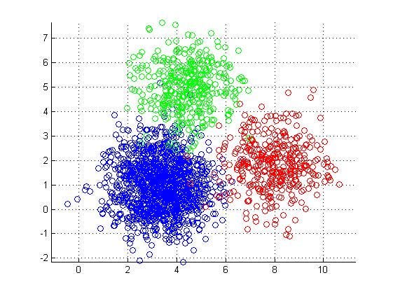
Clustering is a technique that groups similar objects such that the objects in the same group are more similar to each other than the objects in the other groups. The group of similar objects is called a Cluster.
There are 5 popular clustering algorithms that data scientists need to know:
- K-Means Clustering: To know more click here.
- Hierarchical Clustering: We’ll discuss this algorithm here in detail.
- Mean-Shift Clustering: To know more click here.
- Density-Based Spatial Clustering of Applications with Noise (DBSCAN): To know more click here.
- Expectation-Maximization (EM) Clustering using Gaussian Mixture Models (GMM): To know more click here.
Hierarchical Clustering Algorithm
Also called Hierarchical cluster analysis or HCA is an unsupervised clustering algorithm which involves creating clusters that have predominant ordering from top to bottom.
For e.g: All files and folders on our hard disk are organized in a hierarchy.
The algorithm groups similar objects into groups called clusters. The endpoint is a set of clusters or groups, where each cluster is distinct from each other cluster, and the objects within each cluster are broadly similar to each other.
This clustering technique is divided into two types:
- Agglomerative Hierarchical Clustering
- Divisive Hierarchical Clustering
Agglomerative Hierarchical Clustering
The Agglomerative Hierarchical Clustering is the most common type of hierarchical clustering used to group objects in clusters based on their similarity. It’s also known as AGNES (Agglomerative Nesting). It's a “bottom-up” approach: each observation starts in its own cluster, and pairs of clusters are merged as one moves up the hierarchy.
How does it work?
- Make each data point a single-point cluster → forms N clusters
- Take the two closest data points and make them one cluster → forms N-1 clusters
- Take the two closest clusters and make them one cluster → Forms N-2 clusters.
- Repeat step-3 until you are left with only one cluster.
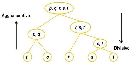
Have a look at the visual representation of Agglomerative Hierarchical Clustering for better understanding:
There are several ways to measure the distance between clusters in order to decide the rules for clustering, and they are often called Linkage Methods. Some of the common linkage methods are:
- Complete-linkage: the distance between two clusters is defined as the longest distance between two points in each cluster.
- Single-linkage: the distance between two clusters is defined as the shortest distance between two points in each cluster. This linkage may be used to detect high values in your dataset which may be outliers as they will be merged at the end.
- Average-linkage: the distance between two clusters is defined as the average distance between each point in one cluster to every point in the other cluster.
- Centroid-linkage: finds the centroid of cluster 1 and centroid of cluster 2, and then calculates the distance between the two before merging.
The choice of linkage method entirely depends on you and there is no hard and fast method that will always give you good results. Different linkage methods lead to different clusters.
The point of doing all this is to demonstrate the way hierarchical clustering works, it maintains a memory of how we went through this process and that memory is stored in Dendrogram.
What is a Dendrogram?
A Dendrogram is a type of tree diagram showing hierarchical relationships between different sets of data.
As already said a Dendrogram contains the memory of hierarchical clustering algorithm, so just by looking at the Dendrgram you can tell how the cluster is formed.
Note:-
- Distance between data points represents dissimilarities.
- Height of the blocks represents the distance between clusters.
So you can observe from the above figure that initially P5 and P6 which are closest to each other by any other point are combined into one cluster followed by P4 getting merged into the same cluster(C2). Then P1and P2 gets combined into one cluster followed by P0 getting merged into the same cluster(C4). Now P3 gets merged in cluster C2 and finally, both clusters get merged into one.
Parts of a Dendrogram
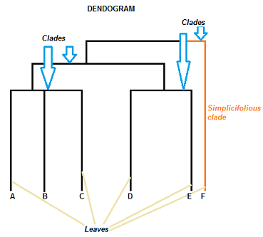
A dendrogram can be a column graph (as in the image below) or a row graph. Some dendrograms are circular or have a fluid-shape, but the software will usually produce a row or column graph. No matter what the shape, the basic graph comprises the same parts:
- The Clades are the branch and are arranged according to how similar (or dissimilar) they are. Clades that are close to the same height are similar to each other; clades with different heights are dissimilar — the greater the difference in height, the more dissimilarity.
- Each clade has one or more leaves.
- Leaves A, B, and C are more similar to each other than they are to leaves D, E, or F.
- Leaves D and E are more similar to each other than they are to leaves A, B, C, or F.
- Leaf F is substantially different from all of the other leaves.
A clade can theoretically have an infinite amount of leaves. However, the more leaves you have, the harder the graph will be to read with the naked eye.
One question that might have intrigued you by now is how do you decide when to stop merging the clusters?
You cut the dendrogram tree with a horizontal line at a height where the line can traverse the maximum distance up and down without intersecting the merging point.
For example in the below figure L3 can traverse maximum distance up and down without intersecting the merging points. So we draw a horizontal line and the number of verticle lines it intersects is the optimal number of clusters.
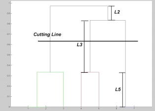
Number of Clusters in this case = 3.
Divisive Hierarchical Clustering
In Divisive or DIANA(DIvisive ANAlysis Clustering) is a top-down clustering method where we assign all of the observations to a single cluster and then partition the cluster to two least similar clusters. Finally, we proceed recursively on each cluster until there is one cluster for each observation. So this clustering approach is exactly opposite to Agglomerative clustering.
There is evidence that divisive algorithms produce more accurate hierarchies than agglomerative algorithms in some circumstances but is conceptually more complex.
In both agglomerative and divisive hierarchical clustering, users need to specify the desired number of clusters as a termination condition(when to stop merging).
Measuring the goodness of Clusters
Well, there are many measures to do this, perhaps the most popular one is the Dunn's Index. Dunn's index is the ratio between the minimum inter-cluster distances to the maximum intra-cluster diameter. The diameter of a cluster is the distance between its two furthermost points. In order to have well separated and compact clusters you should aim for a higher Dunn's index.
Now let's implement one use case scenario using Agglomerative Hierarchical clustering algorithm. The data set consist of customer details of one particular shopping mall along with their spending score.
You can download the dataset from here.
Let's start by importing 3 basic libraries:
import numpy as np
import matplotlib.pyplot as plt
import pandas as pd
Load the dataset:
dataset = pd.read_csv('/.../Mall_Customers.csv')
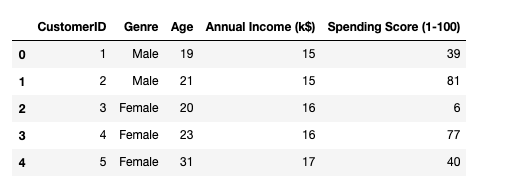
So our goal is to cluster customers based on their spending score.
Out of all the features, CustomerID and Genre are irrelevant fields and can be dropped and create a matrix of independent variables by select only Ageand Annual Income.
X = dataset.iloc[:, [3, 4]].values
Next, we need to choose the number of clusters and for doing this we’ll use Dendrograms.
import scipy.cluster.hierarchy as sch
dendrogrm = sch.dendrogram(sch.linkage(X, method = 'ward'))
plt.title('Dendrogram')
plt.xlabel('Customers')
plt.ylabel('Euclidean distance')
plt.show()

As we have already discussed to choose the number of clusters we draw a horizontal line to the longest line that traverses maximum distance up and down without intersecting the merging points. So we draw a horizontal line and the number of verticle lines it intersects is the optimal number of clusters.
In this case, it's 5. So let's fit our Agglomerative model with 5 clusters.
from sklearn.cluster import AgglomerativeClustering
hc = AgglomerativeClustering(n_clusters = 5, affinity = 'euclidean', linkage = 'ward')
y_hc = hc.fit_predict(X)
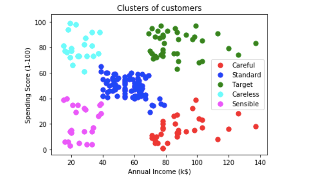
Visualize the results.
# Visualising the clusters
plt.scatter(X[y_hc == 0, 0], X[y_hc == 0, 1], s = 50, c = 'red', label = 'Careful')
plt.scatter(X[y_hc == 1, 0], X[y_hc == 1, 1], s = 50, c = 'blue', label = 'Standard')
plt.scatter(X[y_hc == 2, 0], X[y_hc == 2, 1], s = 50, c = 'green', label = 'Target')
plt.scatter(X[y_hc == 3, 0], X[y_hc == 3, 1], s = 50, c = 'cyan', label = 'Careless')
plt.scatter(X[y_hc == 4, 0], X[y_hc == 4, 1], s = 50, c = 'magenta', label = 'Sensible')
plt.title('Clusters of customers')
plt.xlabel('Annual Income (k$)')
plt.ylabel('Spending Score (1-100)')
plt.legend()
plt.show()
Conclusion
Hierarchical clustering is a very useful way of segmentation. The advantage of not having to pre-define the number of clusters gives it quite an edge over k-Means. However, it doesn't work well when we have huge amount of data.
Well, this comes to the end of this article. I hope you guys have enjoyed reading it. Please share your thoughts/comments/doubts in the comment section.
You can reach me out over LinkedIn for any query.

Thanks for reading !!!
Bio: Nagesh Singh Chauhan is a Big data developer at CirrusLabs. He has over 4 years of working experience in various sectors like Telecom, Analytics, Sales, Data Science having specialisation in various Big data components.
Original. Reposted with permission.
Related:
- Predict Age and Gender Using Convolutional Neural Network and OpenCV
- Introduction to Image Segmentation with K-Means clustering
- Classifying Heart Disease Using K-Nearest Neighbors