A Guide to Automated Deep/Machine Learning for Natural Language Processing: Text Prediction
This article was published as a part of the Data Science Blogathon
This article starts by discussing the fundamentals of Natural Language Processing (NLP) and later demonstrates using Automated Machine Learning (AutoML) to build models to predict the sentiment of text data. Other applications of NLP are for translation, speech recognition, chatbot, etc. You may be thinking that this article is general because there are many NLP tutorials and sentiment analyses on the internet. But, this article tries to show something different. It will demonstrate the use of AutoKeras as an AutoML to generate Deep Learning to predict text, especially sentiment rating and emotion. But before that, let’s briefly discuss basic NLP because it supports text sentiment prediction.
This article will cover the following topics:
- Regular expression
- Word tokenization
- Named Entity Recognition
- Stemming and lemmatization
- Word cloud
- Bag-of-words (BoW)
- Term Frequency — Inverse Document Frequency (TF-IDF)
- Sentiment analysis
- Text Regression (Automated Machine Learning and Deep Learning)
- Text Classification (Automated Deep Learning)
NLP aims to make the sense of text data. The examples of text data commonly analyzed in Data Science are reviews of products, posts from social media, documents, etc. Unlike numerical data, text data cannot be analyzed with descriptive statistics. If we have a list of product prices data containing 1000 numbers, we can understand the overall prices data by examining the average, median, standard deviation, boxplot, and other technics. We do not have to read all the numbers to understand them.
Now, if we have thousands of texts reviewing products from an e-commerce online store, how do we know what the reviews are saying without reading them all. With NLP, those text reviews can be interpreted into satisfaction rating, emotion, etc. This is called sentiment analysis. Machine Learning models are created to predict the sentiment of the text.
Before getting into the sentiment analysis, this article will start from the very basics of NLP, such as regular expression, word tokenization, until Bag-of-Words and how they contribute to the sentiment analysis. Here is the Python notebook supporting this article.
Regular Expression
Regular Expression (RegEx) is a pattern to match, search, find, or split one or more sentences or words. The following code is an example of using 6 RegEx lines to match the same sentence. The RegEx w+, d+, s, [a-z]+, [A-Z]+, (w+|d+) has the code to search for word, digit, space, small-cap alphabet, big-cap alphabet, and digit respectively. The re.match will return the respective text with a certain pattern for the first word of the text. In this case, it is the word “The”.
Notice that the second, third, and fourth returns “None” as the word “The” does not start with a digit, space, and small alphabet.
The RegEx re.search searches the first text according to the pattern. Unlike re.match which only checks the first word in the text, re.search can identify the words after the first word in the text.
print(re.search('w+', text)) # word
print(re.search('d+', text)) # digit
print(re.search('s', text)) # space
print(re.search('[a-z]+', text)) # small caps alphabet
print(re.search('[a-z]', text)) # small caps alphabet
print(re.search('[A-Z]+', text)) # big caps alphabet
print(re.search('(w+|d+)', text)) # word or digit
Output
<re.Match object; span=(0, 3), match='The'>
<re.Match object; span=(23, 24), match='7'>
<re.Match object; span=(3, 4), match=' '>
<re.Match object; span=(1, 3), match='he'>
<re.Match object; span=(1, 2), match='h'>
<re.Match object; span=(0, 1), match='T'>
<re.Match object; span=(0, 3), match='The'>
Instead of only matching the beginning of the text, re.findall finds all of the RegEx pattern in the text and store them in a list.
print(re.findall('w+', text)) # word
print(re.findall('d+', text)) # digit
print(re.findall('s', text)) # space
print(re.findall('[a-z]+', text)) # small caps alphabet
print(re.findall('[a-z]', text)) # small caps alphabet
print(re.findall('[A-Z]+', text)) # big caps alphabet
print(re.findall('(w+|d+)', text)) # word or digit
Output:
['The', 'monkeys', 'are', 'eating', '7', 'bananas', 'on', 'the', 'tree']
['7']
[' ', ' ', ' ', ' ', ' ', ' ', ' ', ' ']
['he', 'monkeys', 'are', 'eating', 'bananas', 'on', 'the', 'tree']
['h', 'e', 'm', 'o', 'n', 'k', 'e', 'y', 's', 'a', 'r', 'e', 'e', 'a', 't', 'i', 'n', 'g', 'b', 'a', 'n', 'a', 'n', 'a', 's', 'o', 'n', 't', 'h', 'e', 't', 'r', 'e', 'e']
['T']
['The', 'monkeys', 'are', 'eating', '7', 'bananas', 'on', 'the', 'tree']
re.split searches for the RegEx pattern in the whole text and splits the text into list of strings based on the RegEx pattern.
print(re.split('w+', text)) # word
print(re.split('d+', text)) # digit
print(re.split('s', text)) # space
print(re.split('[a-z]+', text)) # small caps alphabet
print(re.split('[A-Z]+', text)) # big caps alphabet
print(re.split('(w+|d+)', text)) # word or digit
Output:
['', ' ', ' ', ' ', ' ', ' ', ' ', ' ', ' ', '!']
['The monkeys are eating ', ' bananas on the tree!']
['The', 'monkeys', 'are', 'eating', '7', 'bananas', 'on', 'the', 'tree!']
['T', ' ', ' ', ' ', ' 7 ', ' ', ' ', ' ', '!']
['', 'he monkeys are eating 7 bananas on the tree!']
['', 'The', ' ', 'monkeys', ' ', 'are', ' ', 'eating', ' ', '7', ' ', 'bananas', ' ', 'on', ' ', 'the', ' ', 'tree', '!']
Word Tokenization
There are still many RegEx patterns to explore, but this article will continue to word tokenization. Word tokenization splits sentences into words. The below code shows how it is done. Can you tell which RegEx code above can do the same thing?
import nltk
from nltk.tokenize import word_tokenize, sent_tokenize
word_tokenize(text)
Output:
['The', 'monkeys', 'are', 'eating', '7', 'bananas', 'on', 'the', 'tree', '!']
Besides word tokenization, we can also perform sentence tokenization.
text2 = 'The monkeys are eating 7 bananas on the tree! The tree will only have 5 bananas left later. One monkey is jumping to another tree.'
sent_tokenize(text2)
Output:
['The monkeys are eating 7 bananas on the tree!',
'The tree will only have 5 bananas left later.',
'One monkey is jumping to another tree.']
Named Entity Recognition (NER)
After the word tokenization, we can apply NER to it. NER identifies which entity each word is. Please find the example below of how pos_tag from nltk is used to perform NER.
text_tag = word_tokenize(text2)
nltk.pos_tag(text_tag)
Output:
[('The', 'DT'),
('monkeys', 'NNS'),
('are', 'VBP'),
('eating', 'VBG'),
('7', 'CD'),
('bananas', 'NNS'),
('on', 'IN'),
('the', 'DT'),
('tree', 'NN'),
('!', '.'),
('The', 'DT'),
('tree', 'NN'),
('will', 'MD'),
('only', 'RB'),
('have', 'VB'),
('5', 'CD'),
('bananas', 'NNS'),
('left', 'VBD'),
('later', 'RB'),
('.', '.'),
('One', 'CD'),
('monkey', 'NN'),
('is', 'VBZ'),
('jumping', 'VBG'),
('to', 'TO'),
('another', 'DT'),
('tree', 'NN'),
('.', '.')]
Where, DT=determiner, NNS=plural noun, VBP= verb for non-3rd person singular present, VBG= gerund/present participle verb, CD= cardinal digit, IN= preposition/subordinating conjunction, NN=noun, MD=modal verb, RB=adverb, VB=base form verb, and so on.
Another way to perform NER is by using spacy package. Observe the following example of how spacy identifies each word lemmatization, PoS, tag, dep, shape, whether it is an alphabet, and whether it is a stop word. We will discuss lemmatization later. PoS and tag define the part of speech, such as a determiner, noun, auxiliary verb, number, etc. “dep” shows the word dependencies. “shape” shows the word letters in X and x for big capital and small capital letter respectively. “is_alphabet” and “is_stop_words” identify whether the word is an alphabet or stop word respectively.
import spacy
spa = spacy.load("en_core_web_sm")
spa_text = spa(text)
print('text' + 't' + 'lemmatized' + 't' + 'PoS' + 't' + 'tag' + 't' + 'dep' + 't' +
      'shape' + 't' + 'is_alphabet' + 't' + 'is_stop_words')
for word in spa_text:
      print(word.text + 't' + word.lemma_ + 'tt' + word.pos_ + 't' + word.tag_ + 't' + word.dep_ + 't' + word.shape_ + 't' + str(word.is_alpha) + 'tt' + str(word.is_stop))
Output:
text	lemmatized	PoS	tag	dep	shape	is_alphabet	is_stop_words
The	the		DET	DT	det	Xxx	True		True
monkeys	monkey		NOUN	NNS	nsubj	xxxx	True		False
are	be		AUX	VBP	aux	xxx	True		True
eating	eat		VERB	VBG	ROOT	xxxx	True		False
7	7		NUM	CD	nummod	d	False		False
bananas	banana		NOUN	NNS	dobj	xxxx	True		False
on	on		ADP	IN	prep	xx	True		True
the	the		DET	DT	det	xxx	True		True
tree	tree		NOUN	NN	pobj	xxxx	True		False
!	!		PUNCT	.	punct	!	False		False
Stemming and Lemmatization
Stemming and Lemmatization return a word to its simpler root form. Both stemming and lemmatization are similar to each other. To understand the difference, observe the following code. Here, we apply stemming and lemmatization to the word “studies” and they will return different outputs. Stemming returns “studi” as the root form of “studies”. Lemmatization returns “study” as the root form of “studies”. The root form returned by lemmatization has a meaning. The root form of stemming sometimes does not have a meaning. The word “studi” from stemming does not have a meaning. Stemming cannot change the letter “i” from the word “studies”.
# Stemming
from nltk.stem import PorterStemmer
print(PorterStemmer().stem('studies'))
# Lemmatization
from nltk.stem import WordNetLemmatizer
print(WordNetLemmatizer().lemmatize('studies'))
Output:
studi
study
Word Cloud
For this exercise, we are going to use women’s clothing reviews from an e-commerce dataset. The dataset provides the text reviews and the rating score from 1 to 5. We are now trying to understand what the 23,486 reviews were saying. If the reviews are in numbers, we can use descriptive statistics to see the data distribution. But, the reviews are in text form. How to quickly get a summary of the 23,486 reviews text? Reading them one by one is not an efficient solution.
A simple way is to plot the word cloud. Word cloud displays the commonly found words from the whole dataset. A larger font size means more frequently found.
visual_rev = WordCloud().generate(' '.join(data['Review Text']))
plt.figure(figsize=(8,8))
plt.imshow(visual_rev, interpolation='bilinear')
plt.show()
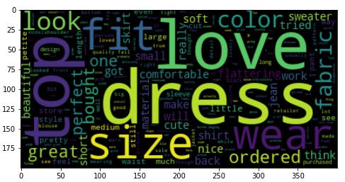
From the word cloud, we can notice that the reviews are talking about dress, love, size, top, wear, and so on as they are the most commonly found words. To display the exact frequency number of each word, we can use Counter(). Let’s demonstrate it using the variable “text2”.
from collections import Counter
Counter(word_tokenize(text2))
Output:
Counter({'The': 2,
'monkeys': 1,
'are': 1,
'eating': 1,
'7': 1,
'bananas': 2,
'on': 1,
'the': 1,
'tree': 3,
'!': 1,
'will': 1,
'only': 1,
'have': 1,
'5': 1,
'left': 1,
'later': 1,
'.': 2,
'One': 1,
'monkey': 1,
'is': 1,
'jumping': 1,
'to': 1,
'another': 1})
The following code does the same thing, but it calls only the top 3 most common words.
Counter(word_tokenize(text2)).most_common(3)
Output:
[('tree', 3), ('The', 2), ('bananas', 2)]
Bag-of-Words (BoW)
Bag-of-Words does a similar thing. It returns a table with features consisting of the words in the reviews. The row contains the word frequency. The following code applies BoW to the women’s clothing review dataset. It will create a data frame with tokenized words as the features.
In the CountVectoricer, I set max_features to be 100 to limit the number of features. “max_df” and “min_df” determine the maximum and minimum appearance percentage of the tokenized words in the documents. The selected tokenized words should appear in more than 10% and less than 95% of the documents. This is to deselect words that appear too rarely and too frequently. “ngram_range” of (1,2) is set to tokenize 1 word and 2 consecutive words (2-word sequence or bi-gram). This is important to detect two-word sequences, like “black mamba”, “land cover”, “not happy”, “not good”, etc. Notice that lemmatizer and regular expression are also used.
# Filter rows with column
data = dataset.loc[dataset['Review Text'].notnull(),:]
# Apply uni- and bigram vectorizer
class lemmatizer(object):
    def __init__(self):
        self.wnl = WordNetLemmatizer()
    def __call__(self, df):
        return [self.wnl.lemmatize(word) for word in word_tokenize(df)]
vectorizer = CountVectorizer(max_features=100, max_df=0.95, min_df=0.1, ngram_range=(1,2),
                             tokenizer=lemmatizer(), lowercase=True, stop_words='english',
                             token_pattern = r'w+')
vectorizer.fit(data['Review Text'])
count_vector = vectorizer.transform(data['Review Text'])

# Transform into data frame
bow = count_vector.toarray()
bow = pd.DataFrame(bow, columns=vectorizer.get_feature_names())
bow.head()
| ! | beautiful | … | ordered | perfect | really | run | size | small | soft | wa | wear | work | |
| 0 | 0 | 0 | … | 0 | 0 | 0 | 0 | 0 | 0 | 0 | 0 | 0 | 0 |
| 1 | 1 | 0 | … | 1 | 0 | 0 | 0 | 0 | 0 | 0 | 0 | 0 | 0 |
| 2 | 1 | 0 | … | 1 | 0 | 1 | 0 | 1 | 3 | 0 | 3 | 0 | 1 |
| 3 | 2 | 0 | … | 0 | 0 | 0 | 0 | 0 | 0 | 0 | 0 | 1 | 0 |
| 4 | 3 | 0 | … | 0 | 1 | 0 | 0 | 0 | 0 | 0 | 0 | 1 | 0 |
| … | … | … | … | … | … | … | … | … | … | … | … | … | … |
Term Frequency — Inverse Document Frequency (TF-IDF)
Similar to BoW, TF-IDF also creates a data frame with features of tokenized words. But, it tries to scale up the rare terms and scale down the frequent terms. This is useful, for example, the word “the” may appear many times, but it is not what we expect as it does not have a sentiment tendency. The values of TF-IDF are generated in 3 steps. Step 1, calculate the TF = count of term/number of words. For example, let’s apply these 3 sentences:
1. The monkeys are small. The ducks are also small.
2. The comedians are hungry. The comedians then go to eat.
3. The comedians have small monkeys.
| Term | TF 1 | TF 2 | TF 3 |
| the | 2/9 | 2/10 | 1/5 |
| monkeys | 1/9 | 0/10 | 1/5 |
| are | 2/9 | 1/10 | 0/5 |
| small | 2/9 | 0/10 | 1/5 |
| ducks | 1/9 | 0/10 | 0/5 |
| comedians | 0/9 | 2/10 | 1/5 |
| hungry | 0/9 | 1/10 | 0/5 |
| … | … | … | … |
The first text contains 9 words. It has 2 words of “the”. So, the word “the” in TF 1 is 2/9.
Step 2, IDF = log (number of documents/number of documents with the term)
| Term | IDF |
| the | log(3/3) |
| monkeys | log(3/2) |
| are | log(3/2) |
| small | log(3/2) |
| ducks | log(3/1) |
| comedians | log(3/2) |
| hungry | log(3/1) |
| … | … |
The word “monkeys” appears 2 times in 3 documents. So, the IDF is log(3/2).
Step 3, calculate the TF-IDF = TF * IDF
| Term | TF 1 | TF 2 | TF 3 | IDF | TF-IDF 1 | TF-IDF 2 | TF-IDF 3 |
| the | 2/9 | 2/10 | 1/5 | log(3/3) |
0.000 |
0.000 |
0.000 |
| monkeys | 1/9 | 0/10 | 1/5 | log(3/2) |
0.020 |
0.000 |
0.035 |
| are | 2/9 | 1/10 | 0/5 | log(3/2) |
0.039 |
0.018 |
0.000 |
| small | 2/9 | 0/10 | 1/5 | log(3/2) |
0.039 |
0.000 |
0.035 |
| ducks | 1/9 | 0/10 | 0/5 | log(3/1) |
0.053 |
0.000 |
0.000 |
| comedians | 0/9 | 2/10 | 1/5 | log(3/2) |
0.000 |
0.035 |
0.035 |
| hungry | 0/9 | 1/10 | 0/5 | log(3/1) |
0.000 |
0.048 |
0.000 |
| … | … | … | … | … | … | … | … |
Here is the output table.
| Term | the | monkeys | are | small | ducks | comedians | hungry | … |
|
1 |
0.000 |
0.020 |
0.039 |
0.039 |
0.053 |
0.000 |
0.000 |
… |
|
2 |
0.000 |
0.000 |
0.018 |
0.000 |
0.000 |
0.035 |
0.048 |
… |
|
3 |
0.000 |
0.035 |
0.000 |
0.035 |
0.000 |
0.035 |
0.000 |
… |
Now, let’s compare it with the BoW data frame below. The word “the” in BoW data frame has the values of 2, 2, and 1 for text 1, 2, and 3 respectively. On the other hand, the same word has 0 value for all of the 3 texts in the TF-IDF data frame. This is because the word “The” appears in all 3 texts. Hence, the IDF is zero (log(3/3)). The words “monkeys” and “ducks” appear once in the first text, but “ducks” has a higher value (0.053) compared to the “monkeys” value (0.020) in the TF-IDF data frame. The word “ducks” appears less in all documents than “monkeys” does, so it gives more highlight to the word “duck”.
| Text | the | monkeys | are | small | ducks | comedians | hungry | … |
| 1 |
2 |
1 |
2 |
2 |
1 |
0 |
0 |
… |
| 2 |
2 |
0 |
1 |
0 |
0 |
2 |
1 |
… |
| 3 |
1 |
1 |
0 |
1 |
0 |
1 |
0 |
… |
Here is the code to apply TF-IDF to the women’s clothing dataset.
from sklearn.feature_extraction.text import TfidfVectorizer
tfidf = TfidfVectorizer(max_features=100)
tfidf.fit(data['Review Text'])
tfidf_data = tfidf.transform(data['Review Text'])

tfidf_data = pd.DataFrame(tfidf_data.toarray(), columns=tfidf.get_feature_names())
tfidf_data.head()
Output:
| all | also | am | an | and | are | … | will | with | work | would | you | |
| 0 | 0.000000 | 0.0 | 0.000000 | 0.0 | 0.602589 | 0.0 | … | 0.0 | 0.000000 | 0.000000 | 0.000000 | 0.0 |
| 1 | 0.000000 | 0.0 | 0.148418 | 0.0 | 0.133039 | 0.0 | … | 0.0 | 0.000000 | 0.000000 | 0.307109 | 0.0 |
| 2 | 0.000000 | 0.0 | 0.000000 | 0.0 | 0.163130 | 0.0 | … | 0.0 | 0.000000 | 0.163481 | 0.000000 | 0.0 |
| 3 | 0.000000 | 0.0 | 0.000000 | 0.0 | 0.142825 | 0.0 | … | 0.0 | 0.000000 | 0.000000 | 0.000000 | 0.0 |
| 4 | 0.228419 | 0.0 | 0.000000 | 0.0 | 0.082899 | 0.0 | … | 0.0 | 0.273455 | 0.000000 | 0.000000 | 0.0 |
What is the use of text converted into BoW or TF-IDF data frame? It is very important if we want to apply Machine Learning to text data. Machine Learning does not understand text, so the text must be converted into a numeric data frame. One of the common use of Machine Learning for text prediction is sentiment analysis. Sentiment analysis can predict the sentiment of the review text. Instead of reading the reviews one by one, sentiment analysis can convert the text into how satisfied the reviews sound.
Sentiment Analysis
Sentiment analysis can be run by using TextBlob or training a Machine Learning model. TextBlob does not require training. It can tell the polarity and subjectivity of the reviews. The polarity ranges from 1 to -1 expressing positive sentiment to negative sentiment. Here is the code to apply sentiment analysis to the text2 = ‘The monkeys are eating 7 bananas on the tree! The tree will only have 5 bananas left later. One monkey is jumping to another tree.’
from textblob import TextBlob
TextBlob(text2).sentiment
Output:
Sentiment(polarity=-0.0125, subjectivity=0.25)
Now, let’s see how it works on the women’s clothing dataset.
# Applying text blob sentiment
def polarity(t):
    a = TextBlob(t).sentiment
    return a[0]
def subjectivity(t):
    a = TextBlob(t).sentiment
    return a[1]
data['polarity'] = data.apply(lambda t: polarity(t['Review Text']), axis=1)
data['subjectivity'] = data.apply(lambda t: subjectivity(t['Review Text']), axis=1)
data.head()
Output:
| Review Text | Rating | polarity | subjectivity | |
| 0 | Absolutely wonderful – silky and sexy and comf… | 4 | 0.633333 | 0.933333 |
| 1 | Love this dress! it’s sooo pretty. i happene… | 5 | 0.339583 | 0.725000 |
| 2 | I had such high hopes for this dress and reall… | 3 | 0.073675 | 0.356294 |
| 3 | I love, love, love this jumpsuit. it’s fun, fl… | 5 | 0.550000 | 0.625000 |
| 4 | This shirt is very flattering to all due to th… | 5 | 0.512891 | 0.568750 |
The table above displays the first 5 rows of the review text polarity. Examine how the words in “Review Text” return the “polarity”. In the same dataset, the satisfaction rating is also given by each of the reviewers in the feature “Rating”. The “Rating” ranges from 1 to 5. The figure below visualizes the polarity distribution of each rating class. Examine that a higher rating tends to have more positive polarity.
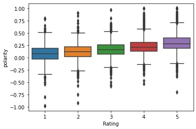
Fig. 2 Polarity distribution of each rating class (source: image by author)
Text Regression (Automated Machine Learning and Deep Learning)
The sentiment analysis provided by TextBlob is a pre-trained model. Users can directly apply it to text. But, what if we want to train our new model to analyze text? What if we want to build a model to detect sentiment ranging from 1 to 5, instead of the text positivity and negativity rate (like using TextBlob)?
Using TextBlob has the advantage that users do not have to train a large number of data. On the other hand, creating a new Machine Learning model for text analysis requires extra time and resources. But, the created new model will be much more customized to a specific topic based on a training dataset. For example, training women’s clothing review dataset will result in an NLP model that is more specific in predicting the sentiment.
In Machine Learning for text analysis or NLP, there are text regression and text classification. Text regression aims to analyze text with continuous or ordinal output. Predicting the “rating” of women’s clothing reviews dataset requires text regression analysis because the output ranges from 1 to 5. The Text Regression notebook is available here.
Just like Machine Learning for structured data, Machine Learning for NLP also requires data frames containing engineered features and label. The engineered features for predictors can be generated using BoW or TF-IDF. The 2 data frames have been made before. According to how the data frames are generated, let’s call them BoW data frame and TF-IDF data frame.
To train a Machine Learning model for text analysis, the technic is the same as training it for structured data. We can use linear regression, decision tree, gradient boosting tree, etc. The code below uses AutoSklearn to train NLP Machine Learning with BoW data frame. AutoSklearn is an automated Machine Learning that can perform feature engineering, model selection, and hyperparameter-tuning automatically. Users can skip those processes and get a model in a specified time allocation. The AutoSklearn below is set to find an optimal model in 3 minutes. To find out more about Automated Machine Learning, visit my previous article.
# Create the model
sklearn = AutoSklearnRegressor(time_left_for_this_task=3*60, per_run_time_limit=60, n_jobs=-1)
# Fit the training data
sklearn.fit(X_train, y_train)
The output prediction of the text regression is a continuous number ranging from 1 to 5. The objective is to predict the review rating ranging from 1 to 5 in integer. So, the predicted values must be rounded to the closest integer between 1 to 5.
# Sprint Statistics
print(sklearn.sprint_statistics())
# Predict the test data
pred_sklearn = sklearn.predict(X_test)
pred_sklearn2 = [round(i) for i in pred_sklearn]
After creating the model, the next step is to validate the model with the unseen dataset. The RMSE of the predicted unseen dataset is 0.9886. However, if we check the prediction outputs with the true values using the confusion matrix, we can find that the model cannot predict well in ratings 1, 2, and 3. Note that this does not necessarily mean that AutoSklearn is not good enough. The AutoSklearn was given only 3 minutes to create models automatically. The result RMSE can be better if it has more time.
# Compute the RMSE
rmse_sklearn = mean_squared_error(y_test, pred_sklearn2)**0.5
print('RMSE: ' + str(rmse_sklearn))
Output:
auto-sklearn results:
  Dataset name: 2fbec688-f37c-11eb-8112-0242ac130202
  Metric: r2
  Best validation score: 0.287286
  Number of target algorithm runs: 27
  Number of successful target algorithm runs: 9
  Number of crashed target algorithm runs: 0
  Number of target algorithms that exceeded the time limit: 9
  Number of target algorithms that exceeded the memory limit: 9
RMSE: 0.9885634389230906
# Prediction results
print('Confusion Matrix')
print(pd.DataFrame(confusion_matrix(y_test, pred_sklearn2), index=[1,2,3,4,5], columns=[1,2,3,4,5]))
Output:
Confusion Matrix
   1  2    3     4     5
1  0  2   66    90     6
2  0  8  132   160    10
3  0  2  177   347    39
4  0  2  136   605   239
5  0  2   79  1170  1257
Let’s repeat the processes above, but this time by using the TF-IDF data frame as the input. AutoSklearn is also applied and the RMSE of the unseen dataset is 0.9770. The result is also similar to the previous one. The predictions are bad in predicting the rating of 1, 2, and 3.
# Create the model
sklearn_idf = AutoSklearnRegressor(time_left_for_this_task=3*60, per_run_time_limit=60, n_jobs=-1)
# Fit the training data
sklearn_idf.fit(X_train_idf, y_train)
# Sprint Statistics
print(sklearn_idf.sprint_statistics())
# Predict the test data
pred_sklearn_idf = sklearn_idf.predict(X_test_idf)
pred_sklearn_idf2 = [round(i) for i in pred_sklearn_idf]
# Compute the RMSE
rmse_sklearn_idf = mean_squared_error(y_test, pred_sklearn_idf2)**0.5
print('RMSE: ' + str(rmse_sklearn_idf))
Output:
auto-sklearn results:
  Dataset name: a573493e-f37f-11eb-8112-0242ac130202
  Metric: r2
  Best validation score: 0.285567
  Number of target algorithm runs: 26
  Number of successful target algorithm runs: 8
  Number of crashed target algorithm runs: 0
  Number of target algorithms that exceeded the time limit: 8
  Number of target algorithms that exceeded the memory limit: 10
RMSE: 0.9769930120276676
# Prediction results
print('Confusion Matrix')
pred_sklearn_idf3 = [i if i <= 5 else 5 for i in pred_sklearn_idf2]
print(pd.DataFrame(confusion_matrix(y_test, pred_sklearn_idf3), index=[1,2,3,4,5], columns=[1,2,3,4,5]))
Output:
Confusion Matrix
   1  2    3     4     5
1  0  3   75    82     4
2  0  5  147   151     7
3  0  6  178   343    38
4  0  1  124   617   240
5  0  0   84  1198  1226
To see which Machine Learning algorithms are created from the AutoSklearn, run the below code.
# Show the models
print(sklearn_idf.show_models())
Now, let’s use another autoML, the AutoKeras. AutoKeras automatically creates Deep Learning models. And yes, not only does it cover the hyperparameter-tuning, but also the Deep Learning layers architecture. After installing and importing the AutoKeras package, we can start the data preparation. The data are prepared in array format separating the training and test datasets. Notice that the feature contains only one column the “Review Text”. AutoKeras does not require users to process applying BoW or TF-IDF. The label is still the same, the “Rating”.
!pip install autokeras
import autokeras as ak
# Preparing the data for autokeras
X_train_ak = np.array(data.loc[X_train.index, 'Review Text'])
y_train_ak = np.array(data.loc[X_train.index, 'Rating'])
X_test_ak = np.array(data.loc[X_test.index, 'Review Text'])
y_test_ak = np.array(data.loc[X_test.index, 'Rating'])
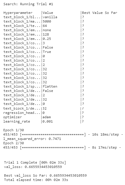
Then, we create a TextRegressor with maximum trials of 3. The AutoKeras will create a maximum of 3 prediction models. The training data is split to have a validation dataset from the 20% of the total training dataset. Then, we can fit the data with 30 epochs for this demonstration.
# Create the model
keras = ak.TextRegressor(overwrite=True, max_trials=3)
# Fit the training dataset
keras.fit(X_train_ak, y_train_ak, epochs=30, validation_split=0.2)
When the AutoKeras is running, it will show the following output cell. But, it will disappear when the process is done.
After the model creation is done, we can export and summarize it. Observe the layers automatically generated by the AutoKeras. The input layer is followed by expand_last_dim, text_vectorization, embedding, dropout, conv1d, max_pooling, flatten, and other layers.
# Show the built models
keras_export = keras.export_model()
keras_export.summary()
Output:
Model: "model"
_________________________________________________________________
Layer (type)                 Output Shape              Param #
=================================================================
input_1 (InputLayer)         [(None,)]                 0
_________________________________________________________________
expand_last_dim (ExpandLastD (None, 1)                 0
_________________________________________________________________
text_vectorization (TextVect (None, 128)               0
_________________________________________________________________
embedding (Embedding)        (None, 128, 128)          640128
_________________________________________________________________
dropout (Dropout)            (None, 128, 128)          0
_________________________________________________________________
conv1d (Conv1D)              (None, 126, 32)           12320
_________________________________________________________________
conv1d_1 (Conv1D)            (None, 124, 32)           3104
_________________________________________________________________
max_pooling1d (MaxPooling1D) (None, 62, 32)            0
_________________________________________________________________
conv1d_2 (Conv1D)            (None, 60, 64)            6208
_________________________________________________________________
conv1d_3 (Conv1D)            (None, 58, 32)            6176
_________________________________________________________________
max_pooling1d_1 (MaxPooling1 (None, 29, 32)            0
_________________________________________________________________
flatten (Flatten)            (None, 928)               0
_________________________________________________________________
dense (Dense)                (None, 32)                29728
_________________________________________________________________
re_lu (ReLU)                 (None, 32)                0
_________________________________________________________________
dense_1 (Dense)              (None, 32)                1056
_________________________________________________________________
re_lu_1 (ReLU)               (None, 32)                0
_________________________________________________________________
dropout_1 (Dropout)          (None, 32)                0
_________________________________________________________________
regression_head_1 (Dense)    (None, 1)                 33
=================================================================
Total params: 698,753
Trainable params: 698,753
Non-trainable params: 0
_________________________________________________________________
Now, let’s see and compare the RMSE of the AutoKeras model. The RMSE is 0.8389. Observing the confusion matrix, the AutoKeras can predict all of the rating levels better. It still cannot predict rating 1 well enough though.
# Predict the test data
pred_keras = keras.predict(X_test_ak)
pred_keras = list(chain(*pred_keras))
pred_keras2 = [i if i <= 5 else 5 for i in pred_keras]
pred_keras2 = [i if i >= 1 else 1 for i in pred_keras2]
pred_keras2 = [round(i) for i in pred_keras2]
# Compute the RMSE
rmse_keras = mean_squared_error(y_test_ak, pred_keras2)**0.5
print('RMSE: ' + str(rmse_keras))
Output:
142/142 [==============================] - 1s 6ms/step
RMSE: 0.8388607442242638
# Prediction results
print('Confusion Matrix')
pd.DataFrame(confusion_matrix(y_test, pred_keras2), index=[1,2,3,4,5], columns=[1,2,3,4,5])
Output:
Confusion Matrix
                1              2              3           4            5
1              20             64             54          23            3
2              20             93            145          49            3
3              11             89            252         166           47
4              2              26            188         423          343
5              0               4            103         676         1725
Text Classification (Automated Deep Learning)
As mentioned before, text classification is another type of text analysis. Emotions detection, movie genres classification, and book types classification are examples of text classification. Unlike text regression, text classification does predict a continuous label, but a discrete label. For this exercise, we are going to use the emotion label dataset. The dataset consists of only two columns: text and label. Our task is to create a prediction model to perceive the emotion of the text. The emotions are classified into 4 classes: anger, fear, joy, and sadness.
For text classification, let’s build two Deep Learning models. The first model applies the technic Long Short-Term Memory (LSTM) model. LSTM model is a Deep Learning model under Recurrent Neural Network (RNN). LSTM is a more advanced model compared to the usual multilayer perceptron Deep Learning. This article will not discuss further RNN or LSTM, but will only apply it for text classification. The LSTM for text classifier notebook is available here.
For data preparation, we apply one-hot-encoding to the data label. It creates 4 columns from 1 label column.
import numpy as np
import pandas as pd
import matplotlib.pyplot as plt
import seaborn as sns
from sklearn.model_selection import train_test_split
from sklearn.metrics import make_scorer, accuracy_score, classification_report, confusion_matrix
# Load dataset
train = pd.read_csv('/content/emotion-labels-train.csv')
test = pd.read_csv('/content/emotion-labels-test.csv')
# Combine training and test datasets
train = pd.concat([train, test], axis=0)
train.head()
| text | label | |
| 0 | Just got back from seeing @GaryDelaney in Burs… | joy |
| 1 | Oh dear an evening of absolute hilarity I don’… | joy |
| 2 | Been waiting all week for this game ❤️❤️❤️ #ch… | joy |
| 3 | @gardiner_love : Thank you so much, Gloria! Yo… | joy |
| 4 | I feel so blessed to work with the family that… | joy |
# One-hot-encoding
trainSet = train.reset_index(drop=True)
labels = pd.get_dummies(trainSet['label'])
trainSet = pd.concat([trainSet, labels], axis=1)
After splitting the training and validation datasets, a tokenizer is applied to tokenize the text. In this demonstration, the tokenizer will keep 5000 most common words. Then, “texts_to_sequences” transforms the texts in the dataset into sequences of integers.
# Split data
X_train, X_val, y_train, y_val = train_test_split(trainSet['text'].values,
                                                  trainSet[['anger','fear','joy','sadness']].values,
                                                  stratify=trainSet['label'],
                                                  test_size=0.2, random_state=123)
# Apply tokenizer and text to sequence
from tensorflow.keras.preprocessing.text import Tokenizer
from tensorflow.keras.preprocessing.sequence import pad_sequences
tokenizer = Tokenizer(num_words=5000, oov_token='x')
tokenizer.fit_on_texts(X_train)
tokenizer.fit_on_texts(X_val)
seq_train = tokenizer.texts_to_sequences(X_train)
seq_val = tokenizer.texts_to_sequences(X_val)
pad_train = pad_sequences(seq_train)
pad_val = pad_sequences(seq_val)
As for the “pad_sequences”, let’s just look at this example.
[
    [17, 154, 3],
    [54, 981, 56, 4],
    [20, 8]
]
is applied with pad_sequences to be
[
    [17 154    3    0],
    [54  981 56    4],
    [20      8    0    0]
]
Observe that the commas are removed and zeros are filled to make all the three lists have the same length.
Next, the code below shows LSTM layers creation using keras.Sequential. The LSTM will accept the input dimension of 5000 which is the number for the 5000 most common words from the tokenizer. After some ‘relu’ activation and dropout layers with several neurons, the last layer has 4 neurons with ‘softmax’ activation. This will classify a text into one of the 4 classes. The LSTM is compiled with ‘categorical_loss entropy’ loss function, ‘adam’ optimizer, and ‘accuracy’ as the scoring metrics.
import tensorflow as tf
from keras.callbacks import EarlyStopping
# Create the model
lstm = tf.keras.Sequential([
    tf.keras.layers.Embedding(input_dim=5000, output_dim=16),
    tf.keras.layers.SpatialDropout1D(0.3),
    tf.keras.layers.LSTM(128),
    tf.keras.layers.Dense(128, activation='relu'),
    tf.keras.layers.Dense(128, activation='relu'),
    tf.keras.layers.Dropout(0.3),
    tf.keras.layers.Dense(128, activation='relu'),
    tf.keras.layers.Dense(64, activation='relu'),
    tf.keras.layers.Dense(64, activation='relu'),
    tf.keras.layers.Dropout(0.2),
    tf.keras.layers.Dense(4, activation='softmax')
])
lstm.compile(loss='categorical_crossentropy', optimizer='adam', metrics=['accuracy'])
The LSTM model will train to find the optimal model in 100 epochs. But, before that, let’s create an early stopping callback. Early stopping is made to avoid spending too much time training the model while the expected target has been achieved or if there is no improvement of the training. In this exercise, the early stopping callback will stop the training before reaching the 100th epochs if a certain target is fulfilled. In this case, I set the target to reach the minimum accuracy of 85.5% for the validation dataset. When this happens, the LSTM model will stop training even though it has not reached 100 epochs. It will also print a message saying that the accuracy has reached more than 85.5%. While fitting the training data, the history is saved in the variable ‘history’.
class earlystop(tf.keras.callbacks.Callback):
  def on_epoch_end(self, epoch, logs={}):
    if(logs.get('val_accuracy')>0.855):
      print("Accuracy has reached > 85.5%!")
      self.model.stop_training = True
es = earlystop()
history = lstm.fit(pad_train, y_train, epochs=100, callbacks=[es],
                   validation_data=(pad_val, y_val), verbose=2, batch_size=100)
Output:
Epoch 1/100
55/55 - 5s - loss: 0.0348 - accuracy: 0.9771 - val_loss: 2.1571 - val_accuracy: 0.8505
Epoch 2/100
55/55 - 5s - loss: 0.0400 - accuracy: 0.9750 - val_loss: 1.9905 - val_accuracy: 0.8460
Epoch 3/100
55/55 - 5s - loss: 0.0386 - accuracy: 0.9728 - val_loss: 2.0930 - val_accuracy: 0.8386
Epoch 4/100
55/55 - 5s - loss: 0.0377 - accuracy: 0.9741 - val_loss: 2.0917 - val_accuracy: 0.8505
Epoch 5/100
55/55 - 5s - loss: 0.0392 - accuracy: 0.9743 - val_loss: 2.1664 - val_accuracy: 0.8431
Epoch 6/100
55/55 - 5s - loss: 0.0377 - accuracy: 0.9739 - val_loss: 1.8948 - val_accuracy: 0.8512
Epoch 7/100
55/55 - 5s - loss: 0.0353 - accuracy: 0.9782 - val_loss: 2.3116 - val_accuracy: 0.8564
Accuracy has reached > 85.5%!
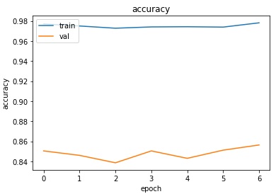
Observe the output cell that the LSTM only runs until the 7th epoch and stops. As we have known, the 7th epoch validation dataset has an accuracy of 85.64%. Examine the training and validation datasets’ accuracy below.
# Visualize LSTM history
plt.plot(history.history['accuracy'])
plt.plot(history.history['val_accuracy'])
plt.title('accuracy')
plt.ylabel('accuracy')
plt.xlabel('epoch')
plt.legend(['train', 'val'], loc='upper left')
plt.show()
Okay, now let’s try to build another model for emotion classification. This time, AutoKeras will be applied. To do this, the code can be similar to the text regressor AutoKeras performed before. Just change the “TextRegressor” into “TextClassifier”, then the rest will work the same. But, the code below will try to perform an advanced text classifier using AutoModel. With AutoModel, we can specify to use TextToIntSequence and Embedding to transform the texts into integer sequences and embed them. We can also specify to use separable convolutional layers. The AutoKeras Text Classifier notebook is available here.
# Create the model
node_input = ak.TextInput()
node_output = ak.TextToIntSequence()(node_input)
node_output = ak.Embedding()(node_output)
node_output = ak.ConvBlock(separable=True)(node_output)
node_output = ak.ClassificationHead()(node_output)
keras = ak.AutoModel(inputs=node_input, outputs=node_output, overwrite=True, max_trials=3)
# Fit the training dataset
keras.fit(X_train_ak, y_train_ak, epochs=80, validation_split=0.2)
# Show the built models
keras_export = keras.export_model()
keras_export.summary()
Output:
Model: "model"
_________________________________________________________________
Layer (type)                 Output Shape              Param #
=================================================================
input_1 (InputLayer)         [(None,)]                 0
_________________________________________________________________
expand_last_dim (ExpandLastD (None, 1)                 0
_________________________________________________________________
text_vectorization (TextVect (None, 64)                0
_________________________________________________________________
embedding (Embedding)        (None, 64, 128)           2560128
_________________________________________________________________
dropout (Dropout)            (None, 64, 128)           0
_________________________________________________________________
separable_conv1d (SeparableC (None, 62, 32)            4512
_________________________________________________________________
separable_conv1d_1 (Separabl (None, 60, 32)            1152
_________________________________________________________________
max_pooling1d (MaxPooling1D) (None, 30, 32)            0
_________________________________________________________________
separable_conv1d_2 (Separabl (None, 28, 32)            1152
_________________________________________________________________
separable_conv1d_3 (Separabl (None, 26, 32)            1152
_________________________________________________________________
max_pooling1d_1 (MaxPooling1 (None, 13, 32)            0
_________________________________________________________________
global_max_pooling1d (Global (None, 32)                0
_________________________________________________________________
dense (Dense)                (None, 4)                 132
_________________________________________________________________
classification_head_1 (Softm (None, 4)                 0
=================================================================
Total params: 2,568,228
Trainable params: 2,568,228
Non-trainable params: 0
_________________________________________________________________
The model has an accuracy of 0.80. Examine the confusion matrix generated below. It shows that the model can predict the emotion based on the text well. To know which emotion is predicted the best, pay attention to the f1-score. Joy has the highest f1-score, followed by fear, anger, and sadness respectively. It means that the model can predict the emotion of joy the best.
# Predict the validation data
pred_keras = keras.predict(X_val_ak)
# Compute the accuracy
print('Accuracy: ' + str(accuracy_score(y_val_ak, pred_keras)))
Output:
25/25 [==============================] - 0s 3ms/step
Accuracy: 0.8042929292929293
# Convert predicted result into pandas series with numeric type
pred_keras_ = pd.DataFrame(pred_keras)
pred_keras_ = pred_keras_[0]
# Prediction results
print('Confusion Matrix')
print(pd.DataFrame(confusion_matrix(y_val, pred_keras_), index=['anger','fear','joy','sad'], columns=['anger','fear','joy','sad']))
print('')
print('Classification Report')
print(classification_report(y_val, pred_keras_))
Output:
Confusion Matrix
       anger  fear  joy  sad
anger    146     6    8   28
fear      16   191    2   43
joy        9     3  166    2
sad       23    12    3  134
Classification Report
              precision    recall  f1-score   support
       anger       0.75      0.78      0.76       188
        fear       0.90      0.76      0.82       252
         joy       0.93      0.92      0.92       180
     sadness       0.65      0.78      0.71       172
    accuracy                           0.80       792
   macro avg       0.81      0.81      0.80       792
weighted avg       0.82      0.80      0.81       792
Conclusion
NLP aims to analyze a large number of text data. Some examples of the applications are for predicting sentiment and emotion from text using Machine Learning. Unlike numerical data, text data need special preprocessing, like BoW or TF-IDF, before fitting them to Machine Learning algorithms.
A regular expression is one of the basic NLP to find and split sentences or words. Word tokenizer splits sentences into words. After that, each tokenized word can be processed with NER, stemming, and lemmatization. Each word is counted for its frequency in the form of a BoW data frame. Stop words that appear frequently, but do not give any meaning, can be removed. Stop words can be identified with NER.
AutoKeras is a package to perform text regression and classification using Deep Learning. Just inputting the text feature will automatically build the model, including word tokenization and preprocessing, hyperparameter-tuning, and deciding the layers.
About Author
Connect with me here.


Hi Rendyk, This is most complete work I find when working with nlp. I think every problem can be solved with this nlp guide when working with text data. Thank you very much for this compiled work !