Gradient Boosting Machine for Data Scientists

Objective

• Boosting is an ensemble learning technique where each model attempts to correct the errors of the previous model.
• Learn about the Gradient boosting algorithm and the math behind it.

Introduction

In this article, we are going to discuss an algorithm that works on boosting technique, The Gradient Boosting algorithm. It is more popularly known as Gradient boosting Machine or GBM.

Note: If you are more interested in learning concepts in an Audio-Visual format, We have this entire article explained in the video below. If not, you may continue reading.

The models in Gradient Boosting Machine are building sequentially and each of these subsequent models tries to reduce the error of the previous model. But the question is how does each model reduce the error of the previous model? It is done by building the new model over errors or residuals of the previous predictions.

This is done to determine if there are any patterns in the error that is missed by the previous model. Let’s understand this through an example.

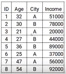
Here we have the data with two features age and city and the target variable is income. So, based on the city and age of the person we have to predict the income. Note that throughout the process of gradient boosting we will be updating the following the Target of the model, The Residual of the model, and the Prediction.

Steps to build Gradient Boosting Machine Model

To simplify the understanding of the Gradient Boosting Machine, we have broken down the process into five simple steps.

Step 1

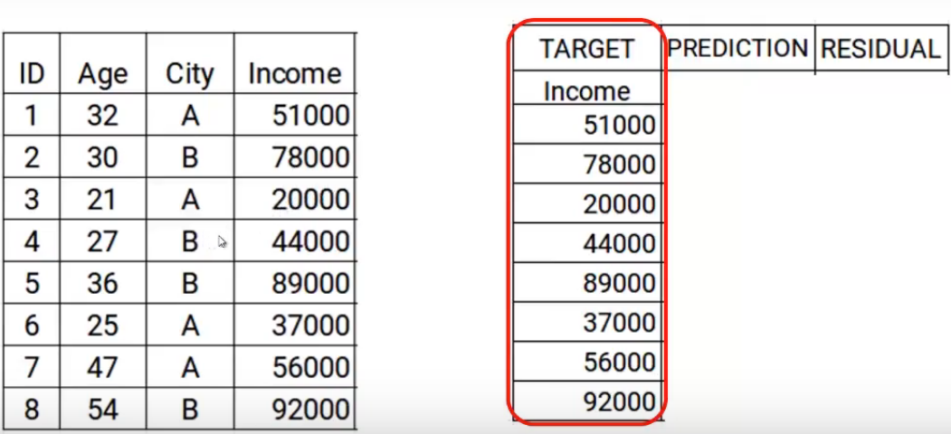
The first step is to build a model and make predictions on the given data. Let’s go back to our data, for the first model the target will be the Income value given in the data. So, I have set the target as original values of Income.

Now we will build the model using the features age and city with the target income. This trained model will be able to generate a set of predictions. Which are suppose as follows.

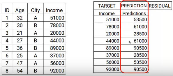
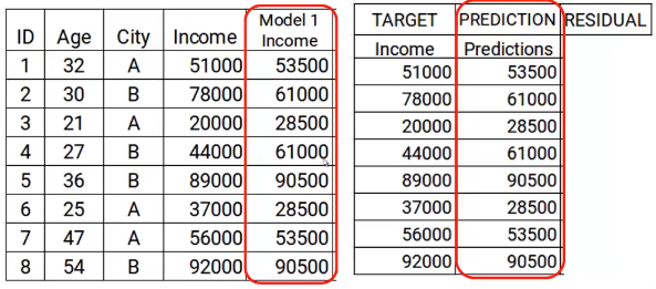
Now I will store these predictions with my data. This is where I complete the first step.

Step 2

The next step is to use these predictions to get the error, which will be used further as a target. At the moment we have the Actual Income values and the predictions from the model1. Using these columns, we will calculate the error by simply subtracting the actual income and the predictions of income. A shown below.

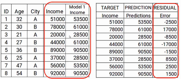
As we mentioned previously the successive models focus on the error. So the errors here will be our new target. That covers up step two.

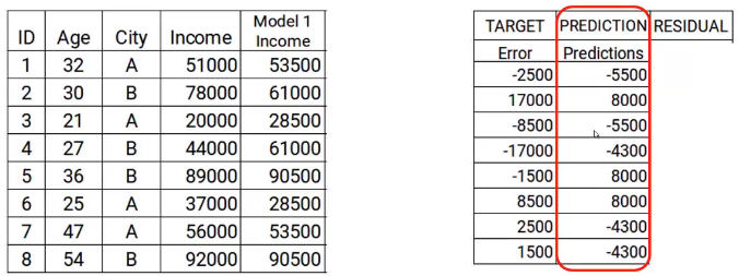
Step 3

In the next step, we will build a model on these errors and make the predictions. Here the idea is to determine, Is any hidden pattern in the error.

So using the error as target and the original features Age and City, we will generate new predictions. Note that the predictions, in this case, will be the error values, not the predicted income values, since our target is the error. Let’s say the model gives the following predictions

Step 4

Now we have to update the predictions of model1. We will add the prediction from the above step and add that to the prediction from model1 and name it Model2 Income.

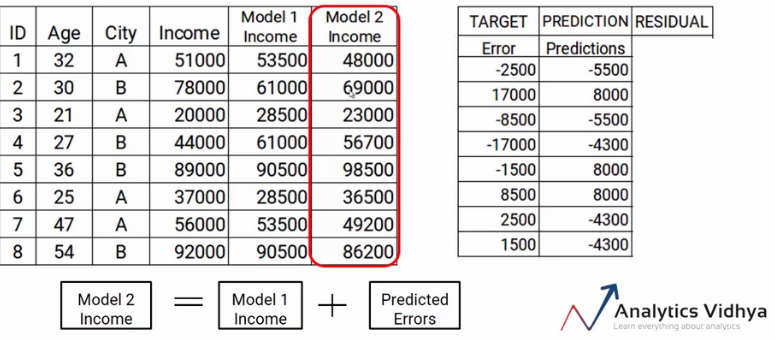
As you can see my new predictions are closer to my actual income values.

Finally, we will repeat steps 2 to 4, which means we will be calculating new errors and setting this new error as a target. We will repeat this process till the error becomes zero or we have reached the stopping criteria, which says the number of models we want to build. That’s the step-by-step process of building a gradient boosting model.

In a nutshell, We build our first model that has features x and target y, let’s called this model H0 that is a function of x and y. Then we build the next model on the errors of the last model and a third model on the errors of the previous model and so on. Till we build n models.

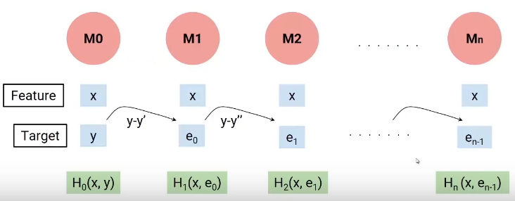
Each successive model works on the errors of all previous models to try and identify any pattern in the error. Effectively, I can say that each of these models is individual functions having independent variable x as the feature and the target is the error of the previous combined model.

So to determine the final equation of our model, we build our first model H0, which gave me some predictions and generated some errors. Let’s call this combined result F0(X).

Now we created our second model and added new predicted errors to F0(X), this new function will be F1(X). Similarly, we will build the next model and so on, till we had n models as shown below.

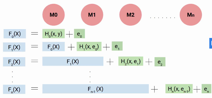
So, at every step, we are trying to model the errors, which helps us to reduce the overall error. Ideally, we want this ‘en’ to be zero. As you can see each model here is trying to boost the performance of the model hence we use the term boost.

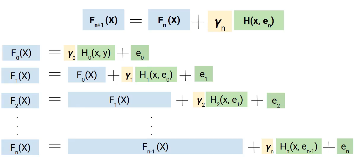
But why we use the term gradient, here is the catch. Instead of adding directly these models, we add them with weight or coefficient, and the right value of this coefficient is decided using the gradient boosting technique.

Hence, a more generalized form of our equation will be as follows.

The math behind Gradient Boosting Machine

I hope, now you have a broad idea of how gradient boosting works. Here onward, we will be focusing on how the value of Yn is calculated.

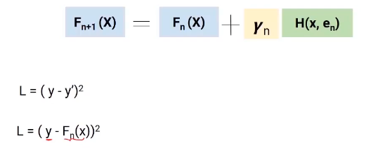
We will use the gradient descent technique to get the values of these coefficients gamma(Y), such that we minimize the loss function. Now let’s dive deeper into this equation and understand the role of the loss function and gamma.

Here, the loss function we are using is (y-y’)2. y is the actual value and y’ is the final predicted value by the last model. So, we can replace y’ with Fn(X) which represents the actual target minus the updated predictions from all the models we have built so far.

Partial Differentiation

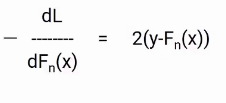
I believe you would be familiar with the gradient descent process as we are going to use the same concept. We will differentiate the equation of L with respect to Fn(X), you will get the following equation, which is also known as pseudo residual. Which is the negative gradient of the loss function.

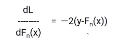
To simplify this, we will multiply both sides with -1. The result will be something like this.

Now, we know the error in our equation of Fn+1(X) is the actual value minus updated predictions from all the models. Hence, we can replace the en in our final equation with these pseudo residuals as shown in the image below.

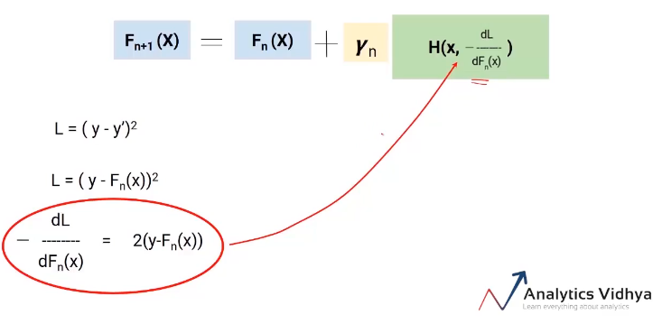
So this is our final equation. The best part about this algorithm is that it gives you the freedom to decide the loss function. The only condition is that the loss function should be differentiable. For ease of understanding, we used a very simple loss function (y-y’)2 but you can change it to a hinge loss or logit loss or anything.

The aim is to minimize the overall loss. Let’s see what would be the overall loss here, it will be the loss up to model n plus the loss from the current model we are building. Here is the equation.

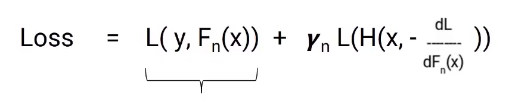
In this equation, the first part is fixed but the second part is the loss from the model we are currently working on. The loss of this model still can not be changed but we can change the gamma value. Now we need to select the value of gamma such that the overall loss is minimized and this value is selected using the gradient descent process.

So the idea is to reduce the overall loss by deciding the optimum value of gamma for each model that we build.

Gradient Boosting Decision Tree

I talk about a special case of gradient boosting i.e Gradient boosting decision tree (GBDT). Here, each model would be a tree and the value of gamma will be decided at each leaf-level, not at the overall model level. So as sown in the following image each leaf would have a gamma value.

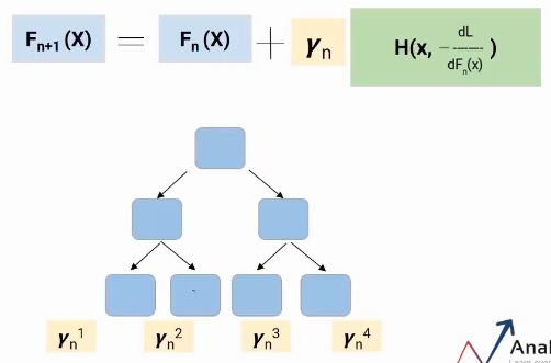
That’s how Gradient Boosting Decision Tree work.

End Notes

Boosting is a type of ensemble learning. It is a sequential process where each model attempts to correct the errors of the previous model. This means every successive model is dependent on its predecessors. In this article, we saw the gradient boosting algorithm and the math behind it.

As we have a clear idea of the algorithm, try to build the models and get some hands-on experience with it.

If you are looking to kick start your Data Science Journey and want every topic under one roof, your search stops here. Check out Analytics Vidhya’s Certified AI & ML BlackBelt Plus Program

If you have any queries let me know in the comment section!

If you have any queries let me know in the comments below!