Predicting SONAR Rocks Against Mines with ML

This article was published as a part of the Data Science Blogathon.

Introduction

This article is about predicting SONAR rocks against Mines with the help of Machine Learning. SONAR is an abbreviated form of Sound Navigation and Ranging. It uses sound waves to detect objects underwater. Machine learning-based tactics, and deep learning-based approaches have applications in detecting sonar signals and hence targets.

Fourier transform, wavelet transform, limit cycle, etc. are signal processing methods applicable for an underwater acoustic signal. Machine Learning enables the processing of sonar signals and target detection. It is a subfield of artificial intelligence which tells machines how to manipulate data more proficiently. The three stages of Machine Learning are taking some data as input, extracting features, and predicting new patterns. The most common ML algorithms in this field are Logistic Regression, support vector machine, principal component analysis, k-nearest neighbors (KNN), C-means clustering, etc.

Let us take the dataset of sonar data and do exploratory data analysis

EDA Exploratory Data Analysis

For any analysis, we need to have data. So, at the outset, we shall import data. Importing of data starts by following lines of code

import numpy as np
import pandas as pd
import matplotlib.pyplot as plt

In the above lines of code, we have imported numpy and pandas libraries respectively. Then, we have imported the matplotlib library which is a detailed library useful for interactive visualizations in python. Next step would be to create a dataframe. Pandas dataframe is a 2-dimensional tabular structure with rows and columns.

df=pd.read_csv('sonar_data.csv',header=None)

The file is in the name output and the above line of code upload data from the external sources. ‘read_csv’ enables us to read csv files. As there is no header row, so header has been passed none option.

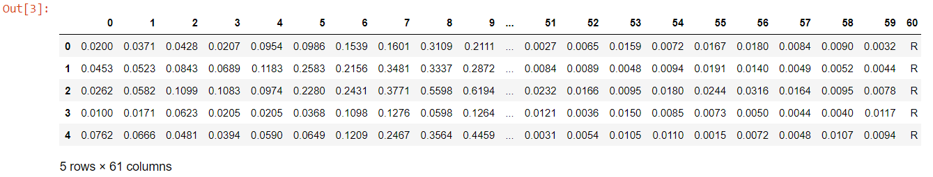
df.head()

The above mentioned code ‘df.head()’ displays the top 5 rows of the dataset as follows

df.shape()

The code written above would display the number of rows and columns in the dataset as follows

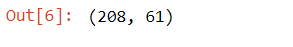
So, there are 208 rows and 61 columns in the dataset.

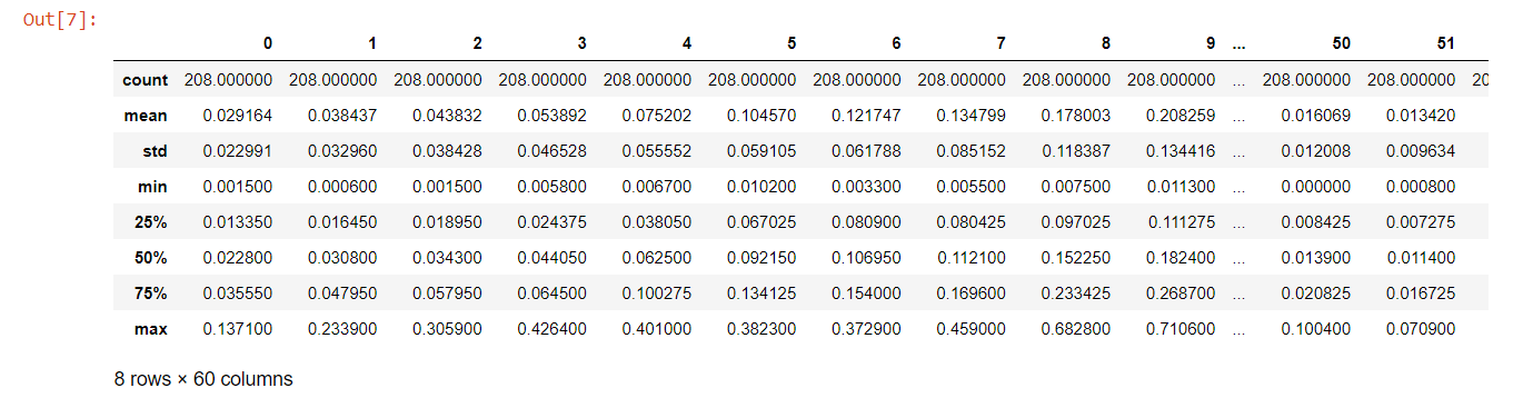
To understand the statistical significance of the dataset, we shall be using ‘describe()’ function. This method would enable the calculation of count, mean, std, min, 25%, 50%, 75%, and a max of the dataset. Count refers to the number of non-empty values; std refers to standard deviation; min is the minimum value, and max is the maximum value. Here, we shall be using ‘T’ function to transpose index and columns of the dataframe.

df.describe()

from sklearn.model_selection import train_test_split
from sklearn.linear_model import LogisticRegression
from sklearn.neighbors import KNeighborsClassifier
from sklearn.metrics import accuracy_score, confusion_matrix

The train_test_split would split arrays or matrices into random train and test datasets. It has been imported from scikit learn library; sklearn.linear_model implements regularized logistic regression using the ‘liblinear’ library; kNN is a non-parametric and lazy learning algorithm and the number of neighbors is the core deciding factor; Accuracy is the number of corrrected predictions divided by total number of predictions, and Confusion matrix is a matrix of size 2×2 for binary classification with the real values on one axis and predicted values on another axis. After importing the necessary dependencies, let us continue with a bit more exploration.
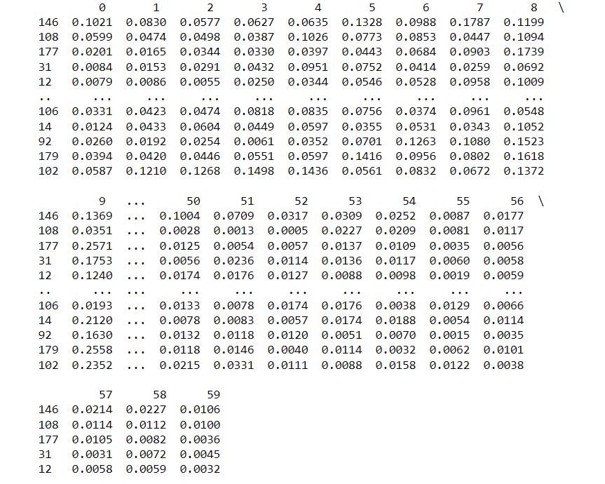
Now the columns have been numbered from 1 to 60. The last column contains values for “R” which denotes rock and “M” which denotes mine. The inputs would range from columns 0 to 59 while column 60 would be the target column. Let’s check the classes balance both in the forms of figure and plot.

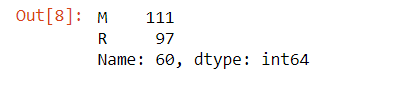
df[60].value_counts()

df[60].value_counts().plot(kind=’bar’)

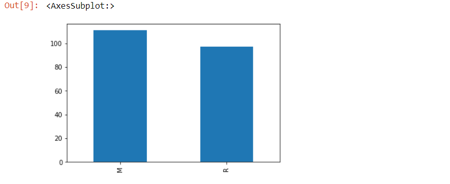
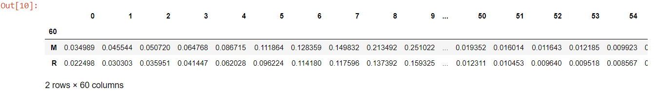
‘M‘ represents mines, and ‘R‘ represents rocks. Both are almost similar in numbers. Now, let us group this data of mines and rocks through the mean function.

Model Development

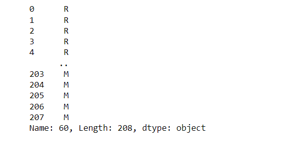
Then, we shall proceed to label the inputs and the output. Here,’Y’ is the target variable and whether the detected substance is rock or mine would be based on the inputs provided.

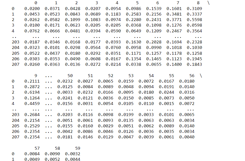
X=df.drop(columns=60,axis=1)
Y=df[60]

Here,’Y’ is the target variable and whether the detected substance is rock or mine would be based on the inputs provided.

print(X)

print(Y)

X_train, X_test, y_train, y_test = train_test_split(X, Y, test_size=0.30, random_state=42)

The above line of code would split the data into train and test datasets to measure the model generalization to predict unseen data of the model. Now, we shall develop the model with the help of 2 different algorithms viz. kNN and Logistic Regression.

Model development with kNN

kNN works by selecting the number k of the neighbors followed by a calculation of Euclidean distance. Then, the number of data points is counted in each category and the new data points are assigned to that category. Let’s look at the lines of code

neighbors = np.arange(1,14)
train_accuracy =np.empty(len(neighbors))
test_accuracy = np.empty(len(neighbors))

Now, we shall fit kNN classifier to the training data

for i,k in enumerate(neighbors):
 knn = KNeighborsClassifier(n_neighbors=k)
 knn.fit(X_train, y_train)
 train_accuracy[i] = knn.score(X_train, y_train)
 test_accuracy[i] = knn.score(X_test, y_test)

Now, we shall plot the number of neighbors against accuracy to select the most suited number of neighbors.

plt.title('k-NN Varying number of neighbors')
plt.plot(neighbors, test_accuracy, label='Testing Accuracy')
plt.plot(neighbors, train_accuracy, label='Training accuracy')
plt.legend()
plt.xlabel('Number of neighbors')
plt.ylabel('Accuracy')
plt.show()

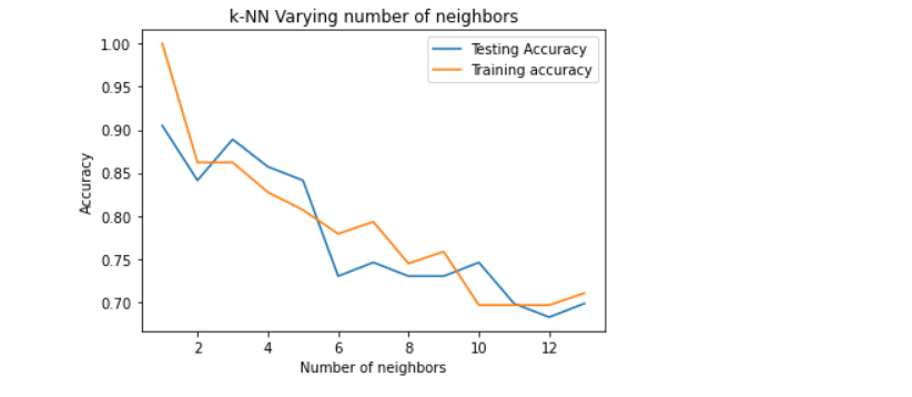
From the above plot, it can be seen that accuracy for both the training as well as the testing data decreases with the increasing number of neighbors, so k=2 would be a safe number to assume.

knn = KNeighborsClassifier(n_neighbors=2)

knn.fit(X_train,y_train)

y_pred = knn.predict(X_test)

Model development with Logistic Regression

We shall perform some more data pre-processing before fitting logistic regression to the training set.

print(X.shape,X_train.shape,X_test.shape)

Through the above line of code, we get to know the number of rows and columns of test and train dataset.

print(X_train)
print(y_train)

Now, we shall fit logistic regression to the training set.

model=LogisticRegression()
model.fit(X_train,y_train)

Evaluation of models through accuracy score and confusion matrix
kNN

knn.score(X_test,y_test)

The model gave us an accuracy score of 84%. For a better understanding of the model, a confusion matrix through frequency tables can be seen.

pd.crosstab(y_test, y_pred, rownames=['True'], colnames=['Predicted'], margins=True)

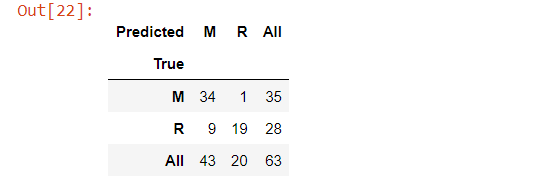
In this model, mines were predicted as mines 34 times, 1-time mines were predicted as rocks, rocks were predicted as mines 9 times, and 19 times rocks were predicted as rocks.

Logistic Regression

score=model.score(X_test,y_test)
print(score)

 

The model gave us an accuracy score of 81%. Confusion matrix can be further seen to understand true positive, false positive, true negative, and false negative.

prediction=model.predict(X_test)

pd.crosstab(y_test, prediction, rownames=['True'], colnames=['Predicted'], margins=True)

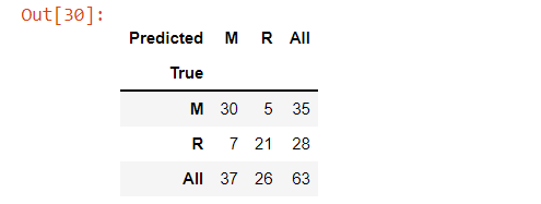
In this model, mines were predicted as mines 30 times, 5 times mines were predicted as rocks, rocks were predicted as mines 7 times, and 21 times rocks were predicted as rocks.

Conclusion

It could be seen that between the 2 models, kNN performed better than Logistic Regression in terms of accurately distinguishing rocks from mines. The ML algorithms in this field that are further recommended are support vector machine, principal component analysis, and C-means clustering.

The media shown in this article is not owned by Analytics Vidhya and is used at the Author’s discretion.