


This post was written by our friends at Insight Data Science. Insight specializes in leveling up the skills of top-tier scientists, engineers, and data professionals, and connects them with companies hiring for roles in data science, engineering, and machine learning to build and scale their tech teams. Their unique approach and rigorous admissions process exposes teams to more highly-qualified talent, saving their partner companies on both the time and cost of hiring.
"God does not play dice." Albert Einstein famously gave this statement in reaction to the emerging theory of quantum mechanics, which seemed to defeat the fundamental laws of physics. Read on to see how the same goes for the fundamental laws of machine learning.
The Classical Bias-Variance-Noise Tradeoff
Before getting into it, let’s briefly review the classical bias-variance-noise tradeoff. The prediction error of a machine learning model, that is, the difference between ground truth and the learned model, is traditionally composed of three parts:
Error = Variance + Bias + Noise
Here, variance measures the fluctuation of learned functions given different datasets, bias measures the difference between the ground truth and the best possible function within our modeling space, and noise refers to the irreducible error due to non-deterministic outputs of the ground truth function itself. If you want to learn more about the bias-variance tradeoff, you can check out this article.
Example: Playing Dice
We are not God — so let’s play some dice! In the following three experiments, we repeat the same steps each time — we roll a die and record the resulting number. The only difference between the experiments is the number of features we are considering.
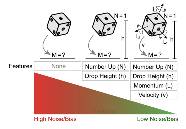
1. No Features
More often than not, rolling a die is associated with generating a random number M between one and six with an equal probability of 16.6%. From this perspective, the output function (the number rolled) is completely non-deterministic, and the error is fully characterized by the noise term.
Error = Noise
Therefore, the expected error and standard deviation are simply those of rolling a die (E = 3.5 and σ = 105/36). Since we are not using any features, there is no model to learn and thus no variance. But is there also no bias?
2. Some Features
Let’s repeat the same experiment, but this time, let’s record the number N facing up at the moment the die is released and the height h it is dropped from. Based on these two features, we can generate pairs of training data x = (h, N) and y = M, where M is the result of the die roll. Armed with enough training data and a good model, we expect that for two new inputs h and N our model is able to predict M better than chance. For example, if N = 1 and h = 5 cm, our model may predict M = 1 with 60% confidence and thus show an improvement over our first model which would have predicted M = 1 with only 16.6% confidence. Thus, we managed to reduce the overall prediction error by reducing the noise term. By training a machine learning model we also introduced a bias and variance term in our overall error.
Error = Variance + Bias + Noise
But didn’t we just repeat the same experiment?
3. All Features
Rolling a die is completely deterministic and there is absolutely no randomness in it. As long as we keep track of all relevant quantities such as initial speed, angular momentum, air resistance, drop height, etc., we can predict the outcome of the roll with 100% accuracy. We don’t even need a machine learning model to predict the outcome. Instead, we can apply the laws of physics. But the laws will get complicated, so for the sake of our example, let’s train a machine learning model instead. In this case, we expect that noise is completely eliminated and we are left with just bias and variance.
Error = Variance + Bias
If we consider a very complex (and suitable) modeling space, we will have almost no bias. If we further assume a huge amount of training data, our variance will also be very small. In such a case, our overall prediction error will be close to zero.
Putting It All Together
In each of the three experiments above, we threw a single die. Nonetheless, in the first example, our “irreducible error” (or noise) was very large, whereas in the last example it was completely gone. How is that possible?
The answer is simple: there is no such thing as “irreducible error”. When we threw the die in the first experiment, we simply ignored most of our reality. It was ignorance in our experimental design that led to this apparent noise in our output. In the last experiment, in contrast, our awareness was at 100%, and with all that information, we eliminated the apparent noise. But of course, each time the reality was the same; all that changed was our perspective (or bias) when observing the rolling die.
Put differently, noise is never inherent to any observed phenomena but is merely a consequence of an observer’s bias to not collect enough features.
Practical Implications
The above thought experiment may seem purely academic, but it has important practical implications.
When training a machine learning model, we often apply tricks and tips that help reduce bias or variance, and reducing one often increases the other. But what about noise? Is it more like bias or more like variance, and which techniques should we apply to reduce it? The answer is: noise is bias! Therefore, the same techniques that reduce bias also reduce noise, and vice versa.
In particular, techniques that reduce variance such as collecting more training samples won’t help reduce noise. Instead, adding more features and considering more complex models will help reduce both noise and bias.
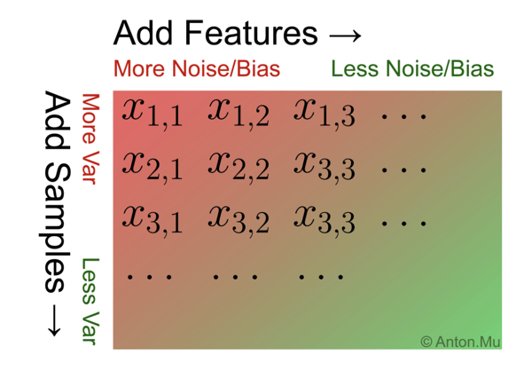
For illustration, let’s arrange our training samples in a matrix form, with each row representing one training sample and each column representing one feature. Extending this matrix on the bottom by adding more training samples will reduce variance. Extending this matrix to the right by adding more features will reduce noise and bias.
Conclusion
In pretty much all practical situations, we find ourselves in the second scenario where we have some (but not all) possible features and thus have some apparent noise. The takeaway is not that (apparent) “noise” doesn’t exist but rather that “noise” is a misleading term. Perhaps it would be more honest to call it “feature bias,” as it stems from our bias of ignoring parts of reality. In this language, what is classically called “bias” should really be called “modeling bias,” as it stems from our particular choice of one model over another.
Next time you face a machine learning problem and find yourself trying to reduce “noise”, pause for a second and ask yourself if you aren’t, in fact, after bias.