Intro to Adversarial Machine Learning and Generative Adversarial Networks

By Andrew Martin, Head of Data at Looka (formerly Logojoy).

Machine learning is an ever-evolving field, so it can be easy to feel like you're out of the loop on the latest developments changing the world this week. One of those emerging areas that have been getting a lot of buzz lately is GANs—or generative adversarial networks.

So to keep you in the machine learning loop, we’ve put together a short crash course on GANs:

• Where they fit into the pantheon of generative models
• How they’ve changed over time
• Where they’re being applied
• Challenges that come with GANs
• What the future has in store for this emerging area of machine learning

Let’s get started.

Generative Models

With generative models, the aim is to model the distribution of a given dataset. For the generative models that we’re talking about today, that dataset is usually a set of images, but it could also be other kinds of data, like audio samples or time-series data.

There are two ways to go about getting a model of this distribution: implicitly or explicitly.

So what’s the difference between the two?

Well, with an explicit generative model, you have the probability density at your disposal. We can model all the variables from that distribution directly. Whereas with an implicit generative model you have to sample in order to get a sense of our model distribution.

When we’re evaluating generative models, one way to do that (which happens to look very good in papers) is using images. So we can sample from our model distribution and then visually inspect the samples to see how well they match up with our original data. The closer our sample images are to our training images, the better our model is.

Types of Generative Models

In the context of deep learning, when we talk about generative models, we’re usually talking about one of four kinds of models:

1. Autoregressive
2. Reversible
3. Variational Autoencoders
4. Generative Adversarial Networks

Autoregressive models: With autoregressive models, you generate an image by generating each pixel conditioned on the previous pixels that you’ve generated. That is to say, when you generate an image using an autoregressive model, you generate it pixel by pixel. Here’s an example of an autoregressive model.

Reversible models: The concept of a reversible model is to take a GAN, but make the generator process reversible. This means we can pass images and noise both ways through a reversible model—going from noise to image and image to noise. This is an example of a reversible model.

Variational Autoencoders:  Autoencoders consist of a pair of connected networks: the encoder and the decoder. Variational autoencoders are distinguished by having a continuous latent space. This allows for easy sampling and interpolation, which is particularly useful when VAEs are used to explore variations on pre-existing data in a specified direction. Here’s a look at a variational autoencoder.

Generative Adversarial Networks

Now, after traversing through other generative models, we get to GANs—or generative adversarial networks.

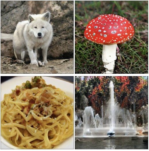
(image from Brock 2018)

To begin, let’s examine some images that have been generated from GANs, to get an idea of how much progress has been made in the last five years. These images above are unconditionally generated ImageNet samples taken from a model called BigGAN which was presented by Andrew Brock at ICLR (International Conference on Learning Representation) in 2019.

These image samples are remarkable for two main reasons: the level of clarity and the diversity of classes. You have an animal, a mushroom, food, a landscape—all generated together, all with clear resolution.

But it wasn't always like this.

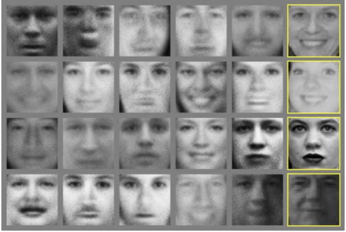
(image examples from Goodfellow et al 2014)

This is an image from the original GAN paper, by Ian Goodfellow et al. in 2014. When this paper came out, this was state of the art image generation. But compared to the samples coming out of BigGAN, they’re worlds apart. Just glancing at these samples generated from the Toronto face data set, you can see the images are very low resolution, with features that aren’t fully resolved.

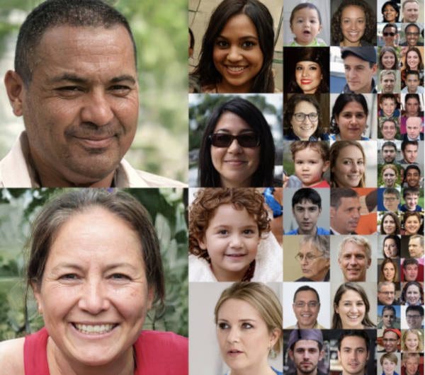
(image examples from Karras et al. 2019)

Now fast forward four years to the StyleGAN paper out of Nvidia, and these generated humans look like they could be real. From fuzzy beginnings in 2014, faces generated by GANs have become almost indistinguishable from real people in just 4 years.

Overview of GANs

Like the other models we discussed, GANs are a form of a generative model. However, unlike the other models we discussed, GAN’s are an implicit generative model. To refresh, this means that if we want to see how good of a model we have of the distribution we have to sample it.

So how do GANs work?

With a GAN we have two networks: a generator (the generative component) and a discriminator (the adversarial component).

The discriminator is trained to identify generated examples and distinguish them from real examples. We train discriminators by taking a set of real examples and a set of generated examples and having the discriminator attempt to classify which examples are real. Through training we want the discriminator to be able to identify whether a sample comes from the real distribution or the generated distribution.

The counterpart to the discriminator is the generator, which takes random noise and learns to transform that random noise into realistic-looking samples—realistic enough to eventually fool the discriminator.

This happens over time, as the generator gets better and better at producing samples that look like the real examples, and the discriminator gets to a point where it's making random guesses as to whether a sample was real or generated. We can think of this as a two-player minimax game, and this point where the discriminator is making random guesses is its Nash equilibrium.

Training the GAN Generator

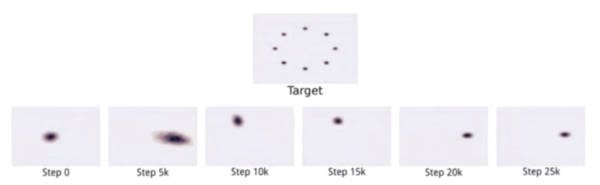
Going into the training a bit more, how exactly does the generator learn to transform random noise into images that can get past the discriminator?

The generator takes samples—typically from a Gaussian— and transforms it through a neural network to create a sample. Again, the goal is to make this sample look as real as possible.

Initially, those transformations really are totally meaningless. So you pass the random noise through the generator, and what you get on the other side looks a lot like random noise.

(illustration of noise to image transformation process. Noise from Adobe Stock, face from Karras et al. 2018)

Now, when you generate an image of grayscale dots, and you pass it to the discriminator, most of the time the discriminator is going to say this doesn't look like a real example. Using backpropagation, you get a signal sent through the generator that tells the layers in the generator to update their weights based on the poor performance of the sample it just sent to the discriminator.

After these adjustments, more random noise passes through the generator to create a new image to send to the discriminator. This time, the discriminator might be fooled by our sample, because—and this is mostly due to randomness early in the training—the image had some features in it that resembled the real dataset. The generator then gets a signal that says that the last sample performed well, and again it updates its weights accordingly.

Through many, many iterations and with very large numbers of images the generator weights continue to update based on how well they do at tricking the discriminator. If training goes well, the generator can take random noise and turn that into a realistic-looking image.

Both the generator and discriminator can train completely unsupervised using this process, and create great samples—due to the dynamics created by the loss functions.

Loss Functions in GANs

In GANs, both the generator and discriminator each have their own loss functions. While these two different loss functions allow for the unsupervised learning we see with GANs, they also create some challenges in training.

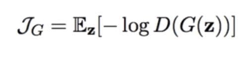
The discriminator’s cost is that it wants to correctly identify real samples as real, and it wants to correctly identify generated samples as generated (equation 1).

(equation 1)

You can see that on the left here, where the first term says to identify real samples as real, and the right term says to identify generated samples as generated.

Now the cool thing here is that the generator cost is just the negative of that function (equation 2).

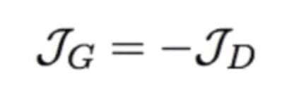
(equation 2)

You'll see here we have a constant for where the equation is referring to the discriminator identifying real examples as real—because the generator is not directly concerned with that part of the process. But what people have found is if they use the loss function for the generator as it is in the top equation, the loss saturates. So what we do is we just change the formulation a bit (equation 3).

(equation 3)

With this version of the loss function, the generator gets very strong signals if it creates samples that the discriminator easily identifies as generated. By using this second equation, it isn't exactly a two-player minimax game formulation anymore, but the training performs as we hope it would—and the training is a lot more stable than it would otherwise be.

Applications of GANs

Now that we’ve got a grasp of training GANs let’s dive into some of the applications.

One of the earliest identified applications GANs comes from Goodfellow’s original paper, which shows interpolating between the numbers 1 & 5 of MNIST. This is a kind of representation learning because through training a generator and discriminator we can learn a latent representation of our original data set.

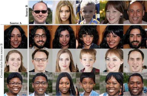
(image from Karras et al. 2019)

You can see the same kind of application in images from the StyleGAN paper (above), as well as many other GAN papers out there.

What we're seeing with this particular example is we're taking the style of source A and applying it to the structure of source B. On the top left we're getting glasses applied to different images or we're making the people on the left look like young children.

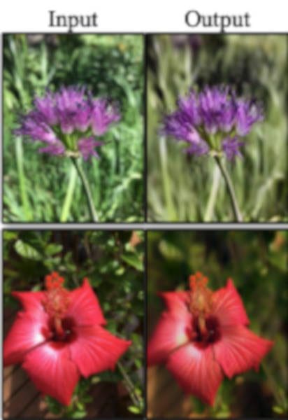
(image examples from Zhu et al. 2017 and Isola et al. 2016)

Another application of GANs is image translation—which in some contexts is a more general approach to style transfer.

On the left (Zhu), we see some image enhancement being done by the CycleGAN, and on the right, in the Pix2Pix paper (Isola), we are translating images from one style to another.

So we have segmentation for the Street View on the left and real images on the right. Then for the aerial to map we have a satellite image and the sort of like map image

What happens when you train this kind of transfer with the Pix2Pix model is you can go satellite to map and map to satellite. So if you’re looking to do style transfer on sets of images, these are the models that work best.

Challenges with GANs

But all the progress with GANs hasn’t come without its challenges.

In theory, GANs operate as this orderly two-player minimax game slowly reaching its Nash equilibrium. We pass noise through the generator, and the generator learns to trick the discriminator, then the discriminator stops being good at detecting the difference and starts randomly guessing, in theory.

There are three main challenges that get in the way of GANs operating as this minimax game:

• Mode collapse
• Finicky training
• Evaluation of GANs

Mode Collapse

(image of mode collapse from Goodfellow 2016)

With mode collapse, the model only learns one or a few of the modes of a multimodal dataset. The data we’re training GANs on typically has a very large number of modes, which makes mode collapse problematic.

Finicky Training

Then there's the issue of finicky training. Earlier, we mentioned the cost functions of the generator and discriminator. And because we have two different cost functions in this model, it creates more challenges in terms of balancing them than you might otherwise have.

Evaluating GANs

When evaluating GANs, several issues come into play.

First, good samples from a generator don't necessarily mean you've learned the distribution well.

Next, it can be very hard to estimate the likelihood, which is a measure of how well you've learned the distribution. Which both lead to the third issue: it's hard to really know how much of the distribution you actually learned.

Finally, evaluating GANs is an active area of research, with no universal method of evaluation. Many papers propose new evaluation metrics that don't receive any attention in future publications.

The Future of GANs

Where do GANs go from here?

We mostly covered GANs generating images in this overview, but that’s far from the only applications of GANs we’re seeing—today or tomorrow.

GANs are also making leaps in things like generating audio for voice impersonations, developing new pharmaceuticals, designing floor plans for buildings, generating components for structures, creating graphic design layouts, generating tabular data, and more.

As this class of machine learning models continues to grow and develop across different industries and applications, and people continue to get more comfortable with the concept of GANs, they’ll continue to find more areas to apply the learnings to. So from 2014 to today and beyond, GANs still have a long way to go before we’ve exhausted all the opportunities that come along with this elegant adversarial system.

 

Bio: Andrew Martin is the Lead Data Scientist at Looka, an AI-powered logo generator that provides business owners with a quick and affordable way to create a beautiful brand. Andrew previously founded Eco Modelling, a consultancy delivering data solutions to clients in forestry and energy. He holds a MSc in Industrial Engineering from Dalhousie University and a BSc in Math from McGill University.

Related:

• Generative Adversarial Networks – Key Milestones and State of the Art
• The Rise of Generative Adversarial Networks
• Why Machine Learning is vulnerable to adversarial attacks and how to fix it