


Using RNNs & DeepAR Models to Find Out
Time series forecasting use cases are certainly the most common time series use cases, as they can be found in all types of industries and in various contexts. Whether it is forecasting future sales to optimize inventory, predicting energy consumption to adapt production levels, or estimating the number of airline passengers to ensure high-quality services, time is a key variable.
And, yet, dealing with time series can be challenging. The data, which consists of sequences of observations recorded at regular time intervals, may contain noise, be highly lumpy, or even be intermittent depending on the context.
Traditional approaches can be over-simplistic and require time-consuming pre and post-processing steps to ensure satisfying performance results.
- In fact, classic time series models usually learn from past observations and therefore predict future values using solely recent history. These models include Autoregression (AR), Moving Average (MA), Autoregressive Integrated Moving Average (ARIMA), and Simple Exponential Smoothing (SES).
- Moreover, the parameters are estimated independently for each time series without taking advantage of the potential positive effects of cross-learning.
- Finally, in an attempt to account for some determinant factors, such as autocorrelation structure, trends, seasonality, and other explanatory variables, approaches consist of selecting the best model for each time series or group of time series and require us to define heuristics, manual interventions, and fine-tuning steps.

These limitations represent the main obstacles to the wide-scale adoption of these approaches.
Meanwhile, over the last few decades, deep learning models have seen great success. Their application to use cases related to natural language processing (NLP), image classification, or audio modeling has consistently outperformed traditional approaches and disrupted business habits. As for time series forecasting, many research papers have successfully applied deep learning methods. They have proposed models that are able to not only overcome the issues encountered with statistical approaches, but better handle the complexity of time series forecasting and, thus, obtain significantly improved results.
Objective
This article is the first of a two-part series that aims to provide a comprehensive overview of the state-of-art deep learning models that have proven to be successful for time series forecasting.
This first article focuses on RNN-based models Seq2Seq and DeepAR, whereas the second explores transformer-based models for time series. Each article compares these models to the standard statistical models.
After reading this series, you will understand:
- What concepts and principles are these models commonly based on?
- How do these models differ from one another?
- To what extent do they provide better results in terms of forecasting accuracy and computing time?
As an illustrative use case, I will rely on the example of the prediction of daily stock market prices of several companies from different industries over a time window of 30 days. This will provide an opportunity to evaluate and compare the performance of these approaches with a concrete use case based on different criteria.
1. Deep Learning Models: Standing on the Shoulders of RNNs
1.1. Refresher on Recurrent Neural Networks
Recurrent Neural Networks (RNN) are frequently used or included as components of the deep learning frameworks of time series models. This is mainly due to their ability to take into account the sequential nature of time series explicitly and thus learn more efficiently. Why?
To What Extent Are RNNs More Adapted to Time Series?
- First, by definition, RNNs refer to the class of neural networks whose neurons send feedback signals to each other through hidden states, as illustrated in Figure 1.
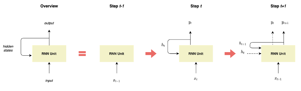
Figure 1: Representation of RNNs, illustration by Lina Faik
- This specific architecture enables RNNs to keep prior inputs “in memory” while predicting the current input and output, contrary to Feed-Forward Neural Networks which consider inputs and outputs as independent of each other.
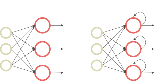
Figure 2: Comparison of Feed-Forward Neural Networks (left) and RNNs (right), illustration by Lina Faik
- Second, RNNs differ from traditional neural networks in terms of the number of parameters to learn. Whereas Feed-Forward Neural Networks have different weights across each node, RNNs share the same parameters within each layer of the network. This is more adapted to sequence data and results in a smaller number of parameters that need to be fitted.
How Do RNNs Process Sequences in Practice?
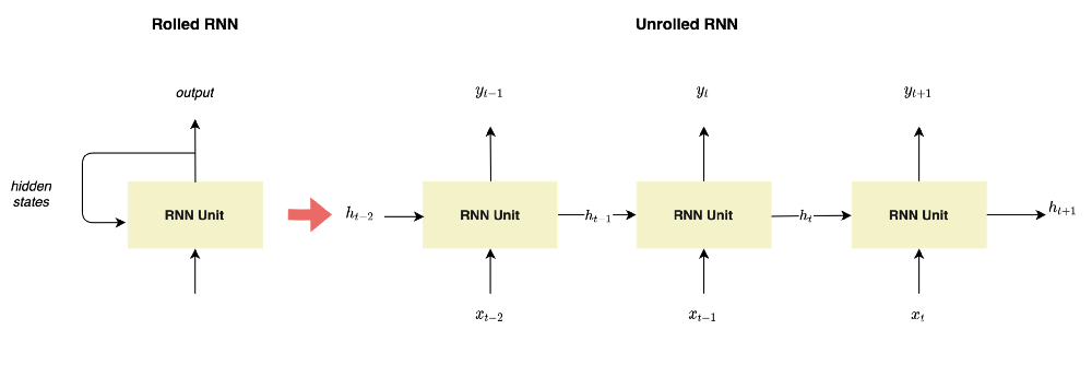
As you can see in the unrolled representation of RNN illustrated in Figure 2, at each time step t, the RNN unit receives the previous hidden states.
What Is Hiding Under These RNN Blocks?
Although not indispensable for the purpose of this article, it can be useful to understand what RNNs consist of by first examining the basic architecture of an RNN cell and then taking a look at some variants.
As illustrated in Figure 4, the standard RNN relies on a simple equation:

where h(t) is the cell’s hidden state at step t and θ is a parameter of a transit function f.
However, because of their recursive nature, RNNs defined as such suffer from technical issues when trained using gradient-based optimization approaches: During the training, the long-term gradients which are back-propagated can tend toward zero and thus vanish or tend toward infinity and thus explode.
In this context, variants of RNNs were introduced to overcome these issues and ended up adding some other interesting properties. These models include Long Short-Term Memory (LSTM) and Gated Recursive Unit (GRU).
For more information, you can read this blog post here or this article here.
1.2 DeepAR
With the availability of large amounts of data comes the need to forecast thousands or millions of related time series. For instance, in the retail industry, retailers are looking to forecast demand for each of their products. In stock markets, brokers need to predict the future stock prices of several companies in order to manage financial portfolios.
Moreover, forecasts depend not only on past values but on other covariates such as dynamic historical features, static attributes for each series, and known future events. And, yet, as classic approaches learn and predict each time series independently, they do not fully leverage cross-learning possibilities or information that may be valuable given the use case.
In this context, DeepAR has proven to be one of the most efficient state-of-the-art forecasting models.
How Does Deep AR Differ From Other Models?
Released by Amazon and integrated into its ML platform SageMaker, DeepAR stands out for its ability to learn at “scale” using multiple covariates.
It consists of a forecasting methodology based on AR RNNs that learn a global model from historical data of all time series in the dataset and produces accurate probabilistic forecasts.
Before diving into how the model works, here are the model’s key advantages:
- Probabilistic forecasting. DeepAR does not estimate the time series’ future values but their future probability distribution. This allows practitioners to compute quantile estimates and thus improves the optimization of business processes. For instance, it enables retailers to better estimate their inventory and brokers to better assess the risk exposure of their portfolio.
- Covariates. DeepAR is able to capture complex and group-dependent relationships by using covariates. It alleviates the efforts and time needed to select and prepare covariates and model section heuristics typically used with classical forecast models.
- Cold-start issues. While traditional methods that predict only one time series at a time fail to provide predictions for items that have little or no history available, DeepAR is able to use learning from similar items to achieve this.
How Does DeepAR Work in Practice?
DeepAR relies on one fundamental idea: Instead of fitting separate models for each time series, it aims to create a global model that learns using all time series in the dataset.
What Is the Architecture of the Model?
Globally, the model consists of a stack of neural networks models, each of them associated with the time series of given item i, y_i.
As shown in Figure 4, these models are composed of RNNs parameterized by Θ_i and a likelihood model p(y_i|θ_i).
The likelihood model should be chosen in accordance with the statistical properties of the data. In the original paper, two likelihood models are considered:
- The Gaussian likelihood parametrized by θ = (μ, σ) where μ is the expected value of the distribution and σ its standard deviation.
- The Negative Binomial likelihood parametrized by θ = (μ, α) where μ is the mean and α its shape.
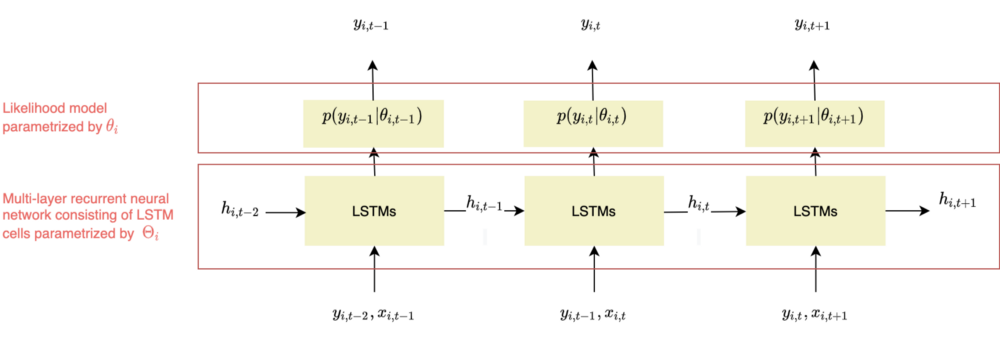
Figure 4 - DeepAR framework, adapted from Salinas, Flunkert, Gasthaus, illustration by Lina Faik
What Are the Different Steps Involved?
As illustrated in Figure 4, at each time step t, the model predicts the following time step t+1 (horizon=1).
The network receives as inputs the last observation y_{i,t-1}, the previous network output h_{i,t-1}, and a set of covariates x_{i,t}. It computes the next hidden states h_{i,t} which is propagated to the hidden layer.

Θ refers to the parameters of the network.
The hidden state is also used to compute the likelihood p(y_{i,t} | θ(h_{i,t}, Θ)) whose parameters are determined by the network output θ(h_{i,t}, Θ). For instance, if the Gaussian likelihood is chosen, the mean μ is computed by using an affine function of the network output and the standard deviation σ is obtained by combining an affine function and a softplus activation (to get a positive value).
As the model aims to learn from all time series simultaneously to leverage the cross-learning effects, its parameters Θ, which consist of both the RNN h(.) and θ(.), are learned by maximizing the log-likelihood over all the items and the entire time range.

The maximization of the log-likelihood can be achieved through stochastic gradient descent by computing gradients with respect to Θ.
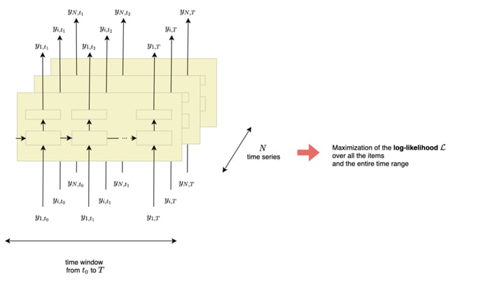 Figure 5 - DeepAR framework, illustration by Lina Faik
How Is DeepAR Trained and Used for Forecasting?
A distinction in the way the model makes predictions should be made between the training and forecasting phases. While in the training phase the values of y_{i,t} are known, during the prediction phase they are unknown for t ≥ t0. Thus, they cannot be used when computing h_{i,t}. To overcome this issue, a sample from the model distribution is used instead.
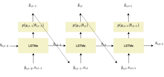
Figure 6 - Forecasting strategy for DeepAR models, adapted from Salinas, Flunkert, Gasthaus, illustration by Lina Faik
Such a learning strategy strongly relates to Teacher Forcing which is commonly used when dealing with RNNs. It refers to the idea of using true values at each new step of the training instead of the model's last predicted outputs.
However, this approach is not without drawbacks. In fact, during training, small mistakes do not contribute significantly to the loss, as the model receives the true value in the next step. As a consequence, the model only learns to predict one time step in advance. However, during forecasts, the model can no longer rely on corrections and has to predict longer sequences. As a consequence, the small mistakes that were not critical during training are now amplified over longer sequences in the forecasting phase.
To sum up, although teacher forcing can enable the model to learn faster and more efficiently, it can also lead to poorer results as training and forecasting become different tasks.
A number of approaches to address this limitation have been proposed. One of them is curriculum learning or scheduled sampling. It consists of randomly or gradually feed the model with its own predicted outputs during the training, rather than the true values.
How Does DeepAR Deal With Heterogeneous Time Series?
Models that try to learn from multiple time series jointly often face two main challenges:
- Scale. Time series can present a wide difference of magnitude. To address this issue, DeepAR computes an item-dependent scale factor ν_i and uses it to rescale the autoregressive inputs y_{i,t}. It also multiplies scale-dependent likelihood parameters by the same factor.

- Imbalanced data. Some items may be underrepresented in the dataset. Usually, a small number of items display a high scale. Therefore, an optimization procedure that simply picks a random sample uniformly would lead the model to underfit these items. This issue is overcome by using a weighted sampling strategy that is dependent of ν_i.
How Does DeepAR Leverage Exogenous Information?
By learning several time series simultaneously, the model is also able to use information from available covariates x_{i,t} and thus leverage cross-learning effectively.
Covariates can be:
- Item-dependent: categorization of item i, for example
- Time-dependent: information about the time point (e.g., week of year)
- Both: price or promotion status for the item i at time t
2. Application to Stock Forecasting
2.1 Scope
It comes as no surprise to anyone that the stock market tends to be very unpredictable. Any change can have a huge impact on stocks trends, whether it’s a major political reversal or a simple Tweet released on the social network platform.
In this context, relying only on financial analysis can be time-consuming and inefficient. Instead, using machine learning can provide better decision support: It can process large chunks of data, learn significant patterns, and spot remarkable opportunities.
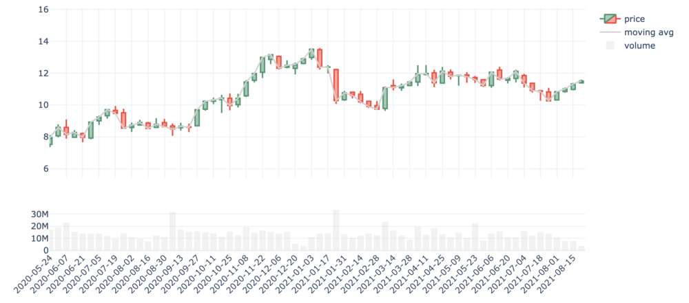
Figure 7 - Evolution of the stock price and trade volumes of EDF
The objective of this section is to compare the performance of deep learning models for time series forecasts to more classical models.
Task: Predict the daily stock prices of large companies over the next 30 days.
About the Dataset
The dataset contains the evolution of the daily stock price of 100 companies randomly chosen from the S&P index over a period of 10 years.
For each company, it also includes information about:
- The industry: ‘Health Care,’ ‘Consumer Discretionary,’ ‘Utilities,’ ‘Financials,’ ‘Information Technology,’ ‘None,’ ‘Industrials,’ ‘Energy’, ‘Real Estate,’ ‘Materials,’ ‘Consumer Staples’
- Its financial data such as: ‘Market Cap,’ ‘EBITDA’
- Its stock performance: ‘Price/Earnings,’ ‘Dividend Yield,’ ‘Earnings/Share,’ ‘52 Week Low’, ‘52 Week High,’ ‘Price/Sales,’ ‘Price/Book’
In addition, features related to dates were also included to take into account weekly, monthly, and yearly seasonalities. For more information, here is an interesting article about how such features can be computed.
Model Benchmark
The performance of the previous model is tested against the following methods:
- Trivial Identity. It relies on recent history to make predictions. This means that it uses the last 30 observations as the forecasts of stock prices over the next 30 days. More information can be found here.
- Seasonal Naive. Similar to the trivial identity approach, it uses recent history to make forecasts but takes seasonality into account. More precisely, supposing a seasonality length h, the forecast in each time step t is:

where T is the forecast time. More information can be found here.
- AutoArima. This algorithm identifies the most optimal parameters for an ARIMA model. It first conducts differentiating tests to define the order of differencing d. Then, it determines the parameters related to seasonality P and Q using the Canova-Hansen to obtain the optimal order of seasonal differencing, D. The best model is chosen based on metrics such as the AIC (Akaike Information Criterion), the BIC (Bayesian Information Criterion), etc. More information about the model can be found here and in the package documentation here.
- Non-Parametric Time Series (NPTS). The idea of this model is to forecast the future value distribution by sampling from past observations. By using an exponential kernel, the model assigns a weight to each of the past observations that decay exponentially according to how far it is from the current time step where the prediction is needed. As a result, recent observations are sampled with a higher probability. More information about the model can be found here.
- Feed-Forward Networks. It trains a simple Multilayer perceptron (MLP) model that predicts the next target time steps given the previous ones. More information can be found here.
Learning Framework
- Training and validation sets. The dataset is split into two: a training dataset that includes all the data except the data related to last to the last 30 days and a validation dataset containing the last 30 days' prices.
- Scenarios. The experimentation includes three different scenarios based on the features used by the model:
Scenario 1. Baseline: Only prices are given to the model.
Scenario 2. Date Features: Besides prices, the model receives features related to the date to take into account weekly, monthly, and yearly seasonality effects.
Scenario 3. Date Features and Covariants: In addition to price and date features, the model is trained using the covariants described above. - Metrics. To compare the performance of the different approaches, I will rely on two metrics: Root-Mean-Square Deviation (RMSE) and Mean Absolute Percentage Error (MAPE) in addition to the computing time used for models to train.
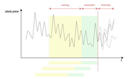 Figure 8 - Learning framework
2.2 Results: Accurate Forecasts and High Potential for Scalability
Overall, the deep learning models outperformed the other models, with the exception of AutoArima. The latter offers comparable prediction accuracy, but it requires a much longer learning time which makes it unscalable in practice.
Table 1 shows the performance metrics for every model in the three scenarios as average over all time series.
Note that these figures should be interpreted with caution: They represent an average. In reality, there is a wide disparity of results depending on the company (the results are strongly dependent on its industry and recent events).
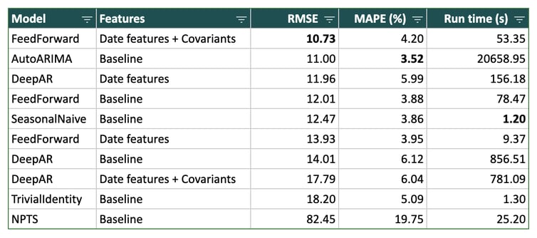 Table 1 - Results (expressed as an average over all time series)
In the rest of this section, you will find my key findings as I explored the results to a more detailed degree:
1. Probabilistic models are more interesting from a business perspective. Since they provide not only forecasts but also uncertainty associated with it, they give an idea of how confident they are about it. In some contexts, this can be crucial.
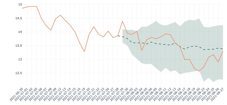 Figure 9 - Forecasts for Ford Motor using DeepAR (baseline), RMSE: 0.17
2. Adding features doesn’t always end up improving results. Figure 10 shows an example of a company for which the results of the model are degraded when trained with covariants.
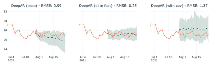 Figure 10: Forecasts for Discovery Communications-C using DeepAR in multiple scenarios
3. Using DeepAR improves results on average, but it is not always the case and depends greatly on the company.
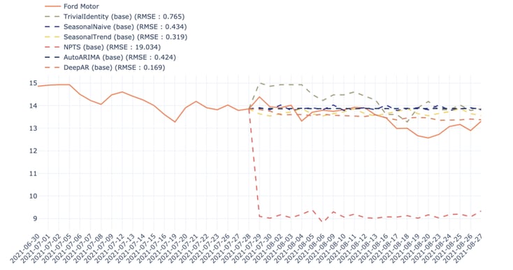 Figure 11: Comparison between different models for the prediction of Ford Motor stock price in the first scenario
It is also worth mentioning that 30 days is a long time period in stock markets.
Conclusion
In this article, we discussed the theoretical principles of Seq2Seq and DeepAR models in the context of time-series predictions. In the next article, we will consider a very popular model in the NLP field: Transformers. We will see how they differ from Seq2Seq and DeepAR models and explore if their adaptation to time series can yield better results.
References:
The experimentations presented above have been carried out in Dataiku using the plugins time series preparation and time series Forecast in addition to Python code. The trained models are based on the library GluonTS except for AutoArima which is based on the Python library pyramid.
[1] D. Salinas, V. Flunkert, J. Gasthaus, DeepAR: Probabilistic Forecasting with Autoregressive Recurrent Networks, April 2017
[2] Z. Tang, P.A. Fishwik, Feedforward Neural Nets as Models for Time Series Forecasting, November 1993
[3] Goodfellow, I., Bengio, Y., & Courville, A. (2016). Deep learning: adaptive computation and machine learning. MIT Press, 2016
[4] A. Amidi, S. Amidi, Stanford CS 230, Deep Learning
[5] J. Brownlee, Multi-Step LSTM Time Series Forecasting Models for Power Usage, October 2018
[6] Tensorflow Tutorials, Time series forecasting