A Comprehensive Guide on Feature Engineering

Why should we use Feature Engineering?

Feature Engineering is one of the beautiful arts which helps you to represent data in the most insightful possible way. It entails a skilled combination of subject knowledge, intuition, and fundamental mathematical skills. You are effectively transforming your data properties into data features when you undertake feature engineering. How you provide your data to your algorithm should effectively denote the relevant structures/properties of the underlying information.

Feature engineering is the process of pre-processing data so that your model/learning algorithm may spend as little time as possible sifting through the noise. Any information that is unrelated to learning or forecasting concerning your final aim is known as noise.

The features you use influence the result more than everything else. No algorithm alone to my knowledge can supplement the information gain given by correct feature engineering.
— Luca Massaron

According to a Forbes poll, data scientists spend 80% of their time preparing data:

This measure demonstrates the significance of feature engineering in data science. As a result, I decided to start this guide, which highlights the key strategies of feature engineering and provides brief descriptions of each.

Iterative steps for Feature Engineering

1. Get deep into the topic, look at a lot of data, and see what you can learn from feature engineering on other challenges.
2. You can make use of automated feature extraction, manual feature construction, or a mixture of the two, depending on your problem.
3. To prepare one or more views for your models to operate on, use various feature importance scores and feature selection approaches.
4. Estimate model accuracy on new data using the features you’ve chosen.

Timestamp

You can decompose a date-time into constituent bits that may help models uncover and exploit links between dates and other variables if you feel it has relationships between them.

The EPOCH time or multiple dimensions is used to represent timestamp information. However, in many applications, much of that data is superfluous. Consider a supervised system attempting to forecast traffic volumes in a city as a function of Location+Time. Trying to learn trends that change by seconds would be primarily misleading in this scenario. The year would also not contribute much to the model’s value. The only measurements you’ll generally need are hours, days, and months. As a result, when representing time, be sure your model requires all of the values you’re giving it.

Consider the following hypothesis: When compared to someone who fills out the same application form in 30 minutes, an applicant who takes days to fill out an application form is likely to be less interested / motivated in the product. Similarly, the amount of time that passes between a bank sending out login data for an online portal and a consumer logging in could indicate a customer’s propensity to use the site. Another example is that a customer who lives closer to a bank branch is more likely to be engaged than a customer who lives further away.

Not to mention time zones. If your data comes from various geographical locations, remember to standardize by time zones if necessary.

Seasonality affects a large number of enterprises. It could be due to tax breaks, the holiday season, or the weather. If this is the case, double-check that the data and variables are for the correct time. For more information, go here.

Missing value treatment for Feature Engineering

Three types of Missing Data are Missing at Random(MAR), Missing Completely at Random(MCAR), Missing Not at Random(MNAR). For brief information go through this.

1. Deletion

Two types: Listwise and Pairwise Deletion.

Listwise: Here, we discard observations in which one or more variables are missing. One of the key advantages of this strategy is its simplicity; nevertheless, because the sample size has reduced, it limits the model’s power.

Pairwise: We undertake analysis for all situations in which the variables of interest are present in pairwise deletion. This strategy has the advantage of keeping as many examples available for study as possible. One of the method’s drawbacks is that various sample sizes had used for different variables.

When the nature of missing data is “Missing fully at random,” deletion methods are applied; otherwise, non-random missing values can bias the model output.

2. Mean/Median/Mode

Imputation is a technique for replacing missing values with estimates. The goal is to use known associations that seem in the valid values of the data set to help estimate the missing values. It is one of the most widely utilized techniques. It entails using the mean, median, or mode to replace missing data for a specific attribute.

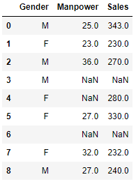
Here, we calculate the mean or median of all non-missing values of that variable and replace the missing values with it. Because variable “Manpower” is missing in the table above, we take the average of all non-missing values of “Manpower” (28.33) and use it to replace the missing value.

round(data['Manpower'].mean(skipna=True),2)

28.33

In this situation, we calculate the average of non-missing values for the genders “Male” (29.33) and “Female” (27.33) separately, then replace the missing value based on gender. We’ll use 29.33 in place of missing “manpower” values for males and 27.33 in place of missing “manpower” values for females.

male =data[data['Gender']=='M']
female =data[data['Gender']=='F']
# mean for male
print(round(male['Manpower'].mean(skipna=True),2))
# mean for female
print(round(female['Manpower'].mean(skipna=True),2))

29.33
27.33

3. Prediction Model

One of the more sophisticated methods for dealing with missing data is the prediction model. Here, we build a predictive model to estimate values that will fill in for missing data. In our case, we split our data set into two sections: one with no missing values for the variable and one with missing values.

The first data set becomes the model’s training data set, and the second data set with missing values becomes the model’s test data set, and missing values are known as the target variable. Then, based on the other attributes of the training data set, we build a model to predict the target variable and populate missing values in the test data set. To accomplish this, we can employ regression, ANOVA, logistic regression, and other modeling techniques. This method has two disadvantages:

• The estimated values of the model are usually better behaved than the real values.
• If there are no relationships between attributes in the data set and the attribute with missing values, the model will be inaccurate in estimating missing values.

4. KNN Imputation

The missing values of an attribute are imputed using the given number of features that are most similar to the feature whose values are missing in this method of imputation. A distance function helps to determine the similarity of two attributes. It is also known to have specific benefits and drawbacks.

Pros

• k-nearest neighbor helps to predict both qualitative and quantitative attributes.
• It is not necessary to create a predictive model for each feature with missing data.
• Features with multiple missing values are simple to handle.
• The data’s correlation structure has been taken into account.

Cons

• When analyzing large databases, the KNN algorithm takes a long time. It searches the entire dataset for the most similar instances.
• The choice of k-value is critical. Here, we include attributes that were significantly different from what we require, in the case of a higher k value. A lower k value implies that significant features are missing.

New ratios

Creating ratios from prior inputs and outputs, rather than merely maintaining them in your dataset, could bring a lot of value. Input/Output (previous performance), productivity, efficiency, and percentages are some of the ratios I’ve utilized in the past. For example, rather than using the total number of cards sold in the branch to predict future credit card sales performance, ratios like credit card sales / Salesperson or credit card sales / Marketing expenditure would be more helpful.

Binning/Bucketing for Feature Engineering

It’s sometimes more intuitive to represent a numerical attribute as a category attribute. By assigning different ranges of a numerical property to different ‘buckets,’ the learning system is subjected to less noise. Consider the challenge of determining whether or not a person owns a specific piece of clothing. There’s a good chance that age is an issue here. The Age Group, on the other hand, is far more important. So, for example, you may have ranges of 1-10, 11-18, 19-25, 26-40, and so on. Furthermore, instead of deconstructing these categories as described in point 2, scalar values could be used because age groups that are ‘near together’ represent similar features.

#Numerical Bin example
Value     Bin
0-30    -> Low
31-70   -> Med
71-100  -> High
#Categorical Bin example
Value       Bin
Spain   -> Europe
Italy   -> Europe
Chile   -> South America

When the domain of your property had separated into clean ranges, where all numbers falling within a limit imply a shared trait, bucketing makes sense. When you don’t want your model to distinguish between values that are too close together, for example, if your property of interest is a function of the entire city, you can aggregate all latitude values inside an area, it decreases overfitting.

Binning reduces the impact of slight mistakes by rounding off a given figure to the nearest representative. If the number of ranges you have is comparable to the total number of potential values, or if precision is crucial, binning isn’t a good idea.

Reframe Numerical Quantities

Your data almost certainly contains quantities that had reframed to reveal needed structures. A translation into a new unit or the breakdown of a rate into time and quantity components are two examples of this.

A quantity could be a weight, a distance, or a time. Regression and other scale-dependent algorithms may benefit from a linear transform.

You might have Item Weight in grams, for example, with a value of 6289. You might make a new feature with this value in kilograms, such as 6.289, or rounded kilos, such as 6. If the domain involves shipping data, kilos might be enough or a better (less noisy) precision for Item Weight.

Item Weight Kilograms and Item Weight Remainder Grams, with example values of 6 and 289, respectively, could be divided into two features: Item Weight Kilograms and Item Weight Remainder Grams.

Domain knowledge may exist that items weighing more than 4 pounds are subject to a higher tax rate. In our case of 6289 grams, that magical domain number had used to create a new binary feature. Item weighing more than 4kg with the value “1.”

You can also store a quantity during an interval as a rate or an aggregate quantity. Number of  Customer Purchases, for example, aggregated over a year.

In this situation, you may wish to return to the data collection process and add more variables to this aggregate, such as seasonality, to show more temporal structure in the purchases. The following new binary features, for example, could be created: Purchases Summer, Purchases Fall, Purchases Winter, and Purchases Spring are the four seasons of purchases.

Transformation for Feature Engineering

Convert complicated non-linear relationships to linear ones. A linear relationship between variables is easy to understand as compared to a non-linear or curved relationship. We can use transformation to turn a non-linear relationship into a linear one. Scatter plots help to figure out how two continuous variables are related. These adjustments also increase the accuracy of the prediction. One of the most prevalent transformation techniques utilized in these scenarios is log transformation.

Symmetric distributions are preferable to skewed distributions because they are easier to read and infer. Some modeling techniques demand that variables have a normal distribution. We can utilize transformations to reduce skewness anytime we have a skewed distribution. We use square/cube root or logarithm of variables for right-skewed distributions and square/cube or exponential of variables for left-skewed distributions.

#Log Transform Example
data = pd.DataFrame({'value':[2,45, -23, 85, 28, 2, 35, -12]})
data['log+1'] = (data['value']+1).transform(np.log)
#Negative Values Handling
#Note that the values are different
data['log'] = (data['value']-data['value'].min()+1) .transform(np.log) 
    value  log(x+1)     log(x-min(x)+1)
0      2   1.09861          3.25810
1     45   3.82864          4.23411
2    -23       nan          0.00000
3     85   4.45435          4.69135
4     28   3.36730          3.95124
5      2   1.09861          3.25810
6     35   3.58352          4.07754
7    -12       nan          2.48491

Cube root helps to calculate negative numbers, including zero. The square root function can be applied to use any positive number, even zero.

Fixing Outliers for Feature Engineering

• A faraway outlier in a sample is an observation that deviates from the broader pattern.
• When looking at the distribution of a single variable, we can detect univariate outliers.
• Outliers in n-dimensional space are multi-variate outliers. One must examine multi-dimensional distributions to locate them.

Types of Outliers

Data Entry: Outliers in data occur by human errors such as those that occur during data collection, recording, or entry. A customer’s annual income is 100,000 Euros. A zero is accidentally added to the figure by the data entry operator. The income has now increased by tenfold to Euros 1,000,000. When compared to the rest of the population, this is an outlier value.

Measurement Error: The most prevalent source of outliers is this. It occurs when the measurement instrument is known to be defective. There are ten weighing machines, for example. One is incorrect, while the other nine are correct. The weight of those who use such equipment will be greater or lower than the rest of the group. Outliers can occur when weights are measured using defective equipment.

Experimental error: It is another source of outliers. Consider the following scenario: In a 100m sprint with seven runners, one runner failed to focus on the ‘Go’ command, causing him to start late. As a result, the runner’s run time was longer than that of other runners. His entire run time may be an aberration.

Intentional: It is typical in self-reported data that contains sensitive information. Teenagers, for example, are prone to underreporting their alcohol consumption. Only a few percentages of them would report the original value. Because the majority of teenagers underreport their use, the accurate figures may appear to be outliers.

Data Preprocessing: We extract data from many sources whenever we execute data mining. Outliers in the dataset could result from data tampering or extraction mistakes.

Sampling: For example, we must determine the height of athletes. We included a couple of basketball players in the sample by accident. Outliers in the dataset are likely as a result of this inclusion.

Natural: When an outlier does not occur by human error, it’s called a natural outlier. Consider the following example: During my most recent work with a reputable insurance business, I found that the top 50 financial counselors outperformed the rest of the population. Surprisingly, it wasn’t because of a mistake. As a result, we take care of this area individually whenever we perform any data mining with advisers.

Many approaches for dealing with outliers are comparable to missing value methods, such as eliminating observations, converting them, binning them, treating them as a separate group, imputing values, and other statistical procedures.

We delete outlier values if they are the result of a data entry error, a data processing error, or if the number of outlier observations is small. Trimming at both ends can also be used to remove outliers.

threshold_value = 0.8

#Dropping columns with missing value rate higher than threshold
data = data[data.columns[data.isnull().mean() < threshold_value]]

#Dropping rows with missing value rate higher than threshold
data = data.loc[data.isnull().mean(axis=1) < threshold_value]

Transforming variables can also reduce outliers. The natural log of a value decreases the variation caused by extreme values. Binning is also a kind of variable transformation. The Decision Tree algorithm enables dealing with outliers well due to binning of a variable. We can also use the method of assigning weights to various observations.

#Numerical Binning Example
data['bin'] = pd.cut(data['value'], bins=[0,30,70,100], labels=["Low", "Mid", "High"]) 
   value   bin
0      2   Low
1     45   Mid
2      7   Low
3     85  High
4     28   Low
#Categorical Binning Example 
     Country
0      Spain
1      Chile
2  Australia
3      Italy
4     Brazil
conditions = [ data['Country'].str.contains('Spain'), data['Country'].str.contains('Italy'),
 data['Country'].str.contains('Chile'),
    data['Country'].str.contains('Brazil')]
choices = ['Europe', 'Europe', 'South America', 'South America']
data['Continent'] = np.select(conditions, choices, default='Other') 
     Country      Continent
0      Spain         Europe
1      Chile  South America
2  Australia          Other
3      Italy         Europe
4     Brazil  South America

Outliers, like missing values, can be replaced. We can use mean, median, and mode imputation methods. Before imputing data, we must determine whether the outlier is natural or artificial. In the case of not ordinary, we can use imputing values. One can further use statistical models to predict the values of outlier observations and then update them with the predicted values.

#filling all missing values with 0
data = data.fillna(0)
# filling missing values with mean of columns
data = data.fillna(data.mean)
# filling missing values with median of columns
data = data.fillna(data.median)

We should treat outliers separately in the statistical model if there are a large number of them. One way is to treat both groups as separate entities, creating individual models for each and combining the results.

Importance of Features in Feature Engineering

An estimate of a feature’s usefulness.

It can be helpful as a starting point for selecting features. Features are assigned scores and can then be ranked based on those scores. The attributes with the highest scores will be included in the training dataset while ignoring the rest.

Feature importance scores can also provide information that you can use to extract or construct new features similar but not identical to those estimated to be helpful.

If a feature had a high correlation with the dependent variable, it might be significant. A few methods include correlation coefficients and other univariate methods.

A few predictive modeling algorithms perform feature importance and selection inside at the time of model construction. MARS, Random Forest, and Gradient Boosted Machines are a few examples. These models can also provide information about the variable importance determined during the model preparation process.

The relative importance of each attribute had computed using decision tree ensemble methods (such as Random Forest or Extra Trees). These essential values help to guide the selection of features.

# Feature Importance
from sklearn import datasets
from sklearn import metrics
from sklearn.ensemble import ExtraTreesClassifier
# load the iris datasets
dataset = datasets.load_iris()
# fit an Extra Trees model to the data
model = ExtraTreesClassifier()
model.fit(dataset.data, dataset.target)
# display the relative importance of each attribute
print(model.feature_importances_)

Output: Below you can see the importance of each attribute.

[ 0.06419645  0.03145001  0.34995716  0.55439638]

Feature Selection

Here, we use specific algorithms to choose a subset of your original features for your final model. You are not creating or modifying your existing attributes in this case but rather pruning them to reduce noise/redundancy.

Feature selection algorithms may use a scoring method, such as correlation or other feature importance methods, to rank and choose features.

More advanced methods may use trial and error to search for subsets of features, automatically creating and evaluating models in search of the objectively most predictive subset of features.

Some methods bake feature selection into the model or obtain it as a side effect of the model. A stepwise regression algorithm is an example that performs feature selection automatically as part of the model construction.

The methods like LASSO and ridge regression are recognized as feature selection algorithms because they actively seek to remove or discount the contribution of features as part of the model building process.

Recursive Feature Elimination (RFE) is a method used for selecting features. This algorithm works by exploring a subset of features from all the available and successfully excluding features until it achieves desired. Fitting the given machine learning algorithm used in the model’s core, ranking features by importance, discarding the least important attributes, and re-fitting the model achieves this. Until we get a specific number of features, the process continues. The model accuracy helps to determine which attributes (and combinations of attributes) contribute the most to predicting the target attribute.

When the full model is created, a measure of variable importance is computed that ranks the predictors from most important to least. At each stage of the search, the least important predictors are iteratively eliminated prior to rebuilding the model.

# Recursive Feature Elimination
from sklearn import datasets
from sklearn.feature_selection import RFE
from sklearn.linear_model import LogisticRegression
# load the iris datasets
dataset = datasets.load_iris()
# create a base classifier used to evaluate a subset of attributes
model = LogisticRegression()
# create the RFE model and select 3 attributes
rfe = RFE(model, 3)
rfe = rfe.fit(dataset.data, dataset.target)
# summarize the selection of the attributes
print(rfe.support_)
print(rfe.ranking_)

[False  True  True  True]
[2 1 1 1]

Feature Standardisation

Many sklearn machine learning algorithms require normalized data, which means zero mean and unit variance. The process of standardization involves rescaling the features so that they have the properties of a standard normal distribution with =0 and =1, where is the mean (average) and is the standard deviation from the mean.

Elements such as the l1 and l2 regularizers in linear models (logistics falls into this category) and the RBF kernel in SVM in the objective function of learners assume that all features are centred around zero and have variance in the same order.

Features with more order of variance might dominate the objective function.

Feature Construction

• Manually creating new features from raw data.
• The best results are achieved by you, the practitioner, modifying the features.
• Feature importance and selection can provide insight into the objective utility of features, but those features must originate somewhere.
• It necessitates spending a significant amount of time with actual sample data (rather than aggregates) and considering the underlying form of the problem, data structures, and how to expose them to predictive modeling algorithms.
• When it comes to tabular data, it usually entails a combination of aggregating or combining features to create new features and decomposing or splitting attributes to generate new ones.
• When dealing with textual data, this frequently entails creating a document or context-specific indicators of a problem relevant. In the case of image data, it is common to spend a significant amount of time defining automatic filters to identify relevant structures.

Pipeline

Scikit-learn’s pipeline module allows you to chain transformers and estimators together so that utilized as a single unit. It comes in handy when you need to jump through a few hoops of data extraction, transformation, and finally train (or use) scikit-learn to generate predictions.

Pipelines assist you in preventing data leakage in your test harness by ensuring that data preparation, such as normalization, is limited to each fold of your cross-validation procedure.

The below is an example of a pipeline with four steps:

# Create a pipeline that extracts features from the data then creates a model
from pandas import read_csv
from sklearn.cross_validation import KFold
from sklearn.cross_validation import cross_val_score
from sklearn.pipeline import Pipeline
from sklearn.pipeline import FeatureUnion
from sklearn.linear_model import LogisticRegression
from sklearn.decomposition import PCA
from sklearn.feature_selection import SelectKBest
# load data
url = "https://archive.ics.uci.edu/ml/machine-learning-databases/pima-indians-diabetes/pima-indians-diabetes.data"
names = ['preg', 'plas', 'pres', 'skin', 'test', 'mass', 'pedi', 'age', 'class']
dataframe = read_csv(url, names=names)
array = dataframe.values
X = array[:,0:8]
Y = array[:,8]
# create feature union
features = []
features.append(('pca', PCA(n_components=3)))
features.append(('select_best', SelectKBest(k=6)))
feature_union = FeatureUnion(features)
# create pipeline
estimators = []
estimators.append(('feature_union', feature_union))
estimators.append(('logistic', LogisticRegression()))
model = Pipeline(estimators)
# evaluate pipeline
num_folds = 10
num_instances = len(X)
seed = 7
kfold = KFold(n=num_instances, n_folds=num_folds, random_state=seed)
results = cross_val_score(model, X, Y, cv=kfold)
print(results.mean())

0.776042378674

Conclusion

I hope you had found this post helpful and insightful. Have a great day.

You can find me on LinkedIn.

Image Source:

• Image 1: Photo by ThisisEngineering RAEng on Unsplash
• Image 2: https://www.forbes.com/sites/gilpress/2016/03/23/data-preparation-most-time-consuming-least-enjoyable-data-science-task-survey-says/
• Image 3: Photo by Javier Huedo on Unsplash
• Image 4: Photo by Chris Lawton on Unsplash
• Image 5: Photo by Will Myers on Unsplash

Pavan Kalyan 27 Oct 2021

Myself Pavan Kalyan with 2 years of experience in developing, deploying scalable Machine Learning models and interested to explore data, discover useful insights. I like to participate in the Machine Hack and Kaggle competitions.