How to Visualize Data in Python (and R)

By SuperDataScience.

At certain cocktail parties, you can get far by arguing that many problems can be reduced, not to data per se, but to its presentation. Brexit? Why it’s the result of a failure to produce compelling, easy-to-understand data visualizations about forecasted quality-of-life changes, you might claim. Or you might propose that Facebook, even by loosey-goosey California standards, is actually in the data-viz game; the data being that of one’s social network made artificially more concrete. Air Quality? Traffic? You might even expound on how proper data visualization is a flexible hammer, and though everything will still look like your thumb, at least you’ll be right.

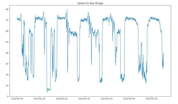
Average speed on the bay bridge over five-minute increments for one week, from one sensor’s point of view (it’s located near Treasure Island). The speed plummets during all reasonable commuting hours, illustrating the law of fixed-supply and demand, which most people call traffic. Made with Matplotlib.

No one said finding these particular cocktail parties would be easy. Or exciting. But either way, being able to produce accessible data visualizations is a key data science skill. So here’s to the data visualizers; those of us who dare to make abstract numbers more immediate, spreadsheets more scintillating (?) and technical reports more manageable. And if you still need more fodder for your cocktail parties, you can name drop W.E. Dubois and Kurt Vonnegut as fellow visualizers, too.

Python and R Walk into a Bar…

The Church-Turing thesis says that what you can do in one program, you can theoretically do in any other. Abstractly, this is true. Practically speaking, however, what is easy to do in one language or software package may take hours of valuable frustration to do in another. (I’m looking at you, Matlab.) Clearly, a lot of these differences have to do with how our brains interact with the programming language, how well we know it, and how well the programming language’s primitives are adapted to the problem at hand. As you are likely aware, the two main general-purpose data programming languages are Python and R, but directly comparing them is unfair. The better comparison is between R and using the Pandas package in conjunction with the Jupyter Notebook. (In the name of full disclosure, I am a member of the “Pandas is generally cooler, unless you have some very specific problems that have not yet been ported to a Python package” camp.).

With that out of the way, the following is what you need to know.

Pandas was first created in 2008, and Python itself was first released in 1991. Many people who use Python claim it is “easy to think in.” R, on the other hand, is actually a mid-90’s implementation of the statistical programming language S, which itself was invented at Bell Labs back in the mid-70s.

But despite the fact that the R governing body is headquartered in Vienna, using it will not make you better at waltzing (indeed, it might make you worse), at eating Manner Wafer cookies, nor will discount tickets to the Vienna Philharmonic appear in your terminal. What can I say, life is tough. Also, a word to the wise: the only way to transfer programming skills to waltzing is to code on ternary computers; both are in base-3. This being said, R is set up to do the kind of data analysis required in laboratory settings producing peer-reviewed material. Given the aforementioned work by Church, Turing as well as by every single open-source contributor, Pandas can do the same thing (just be sure to import statsmodels), generally runs faster, and is easier to optimize (use Numba and Numpy).

In my experience, when used by experts or for niche analyses, R can be a formidable language. However, for the non-experts, R can be harder to audit. For similar reasons, R is also easier to introduce uncaught, silent bugs in one’s data processing pipeline. In other words, this author’s opinion is that it is easier for R code to accumulate technical debt than Python code. On the other hand, it is useful to be able to read R, and clearly this advice changes if you want to work in an R-based shop. Here is a short syntactical comparison between Pandas and R. And if you talk to someone whose primary language is R about this paragraph, they will either enthusiastically admit defeat, or make very reasonable points diametrically opposed to my point of view. Your mileage may vary.

The advice in this article is aimed at the kind of visualization you might to do better understand a dataset, gain insight about it, and communicate results to other people. This is a different purpose than the kind of artistic visualization done by the quality folks at the NYTimes, for instance. (If you are looking to do something that looks as snazzy, you might also want to pick up D3. Or one of the D3 wrappers written in R, or an equivalent in python.)

Lastly, there are a lot of choices. Though the frustrated programmer might disagree with the practical interpretation of the Church-Turing thesis, it is doubly true for data visualization libraries. What good is a data visualization library if it can’t do all of the common visualizations?

General Data Visualization Advice

• Read Tufte.
• Start a new folder whenever you do a new project, download all relevant papers into a research subfolder. (Whatever you are doing, it is helpful to read what has been previously proposed.)
• Start writing the report / whitepaper / paper / summary write-up from the beginning. Take it from someone who has learned this the hard way: saving it for the end is going to engender tons o’ pain; and is likely one reason why certain grad students take forever to finish their thesis.
• Take notes from the beginning too.
• The only people fully qualified enough to write the precise description of what they want are also the sort of people who could do the job.
• Three dimensional images are a separate category unto themselves, but having a Gif of a few 2-D frames stitched together that either vibrate back and forth or change the point of view by a few degrees can make your point.
• Look through Mike Bockstock’s data visualizations and those created by the NYTimes.
• If you have non-technical people who want answers, figure out if it is possible to make the quantitative results follow the visual results. For instance, if there is a way to visualize the results of a clustering analysis, show that before going over any metrics. Concrete is better than abstract, and that’s the point of data visualization.

Specific Data Visualization Advice

• The chroma, “colorfulness” or saturation of a data element can be manipulated to your advantage because Chroma is additive. If two data elements overlap, their saturation can add together to make the overlap literally more vivid. This is a type of “multi-channel reinforcement,” where the fact that two data-points overlap is communicated via both spatial and color channels. In matplotlib, this can be controlled with the alpha
• Perceptually uniform color series can also be used for multi-channel reinforcement, or to add an extra dimension of information to your visualization. For example, the following graphs show Downtown Santa Monica parking lot utilization. In the first, I used the basic colors available, in the second each year is colored via equally-spaced samples of a perceptual color map.

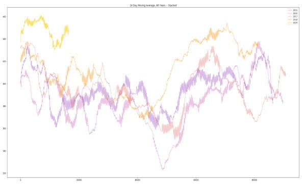
The y-axis shows five 14-day moving averages of the average number of parking spaces available over five-minute increments in the parking lots of Downtown Santa Monica. Higher values mean emptier parking lots, and the ‘0’ on the x-axis corresponds to the first five minutes of each new year. The 2019 line stops at the end of April, and this graph suggests the following conclusion: Retail is dying, long live retail. Made with Matplotlib.

Here is the immediate code I wrote to produce the following plot.  Not shown is the preprocessing I’ve done. I’ve set the “c” parameter to be a perceptual colormap named plasma.

import matplotlib.cm as cm #gets the colormaps

N = 4032 #the number of five minute increments in 14 days

rcParams['figure.figsize'] = 30, 15 #controls a jupyter notebook setting

plt.title("14 Day Moving Average, All Years -- Stacked")

plt.plot(g2015.iloc[N:]['Available'].rolling(N).mean()[N:].values,alpha=.4,c=cm.plasma(1/5,1),label='2015')

plt.plot(g2016.iloc[N:]['Available'].rolling(N).mean()[N:].values,alpha=.4,c=cm.plasma(2/5,1),label='2016')

plt.plot(g2017.iloc[N:]['Available'].rolling(N).mean()[N:].values,alpha=.5,c=cm.plasma(3/5,1),label='2017')

plt.plot(g2018.iloc[N:]['Available'].rolling(N).mean()[N:].values,alpha=.75,c=cm.plasma(4/5,1),label='2018')

plt.plot(g2019.iloc[N:]['Available'].rolling(N).mean()[N:].values,alpha=.9,c=cm.plasma(5/5.5,1),label="2019")

plt.legend()

• Adding dark boundaries around data points can make them look cleaner, and this works if you don’t have a ton of points to visualize, and the points are relatively large. Look for a “edge_colors=True” matplotlib setting.
• One of the lessons from Sparklines is that the human brain can interpret small data elements, especially if what’s important is the macro trend.

Several of these principles are illustrated in the following data visualization. For instance, most of the dots are too small to make out. Also, the saturation or “alpha” property of the color is set to less and 100% so that when the dots overlap they seem to become darker.

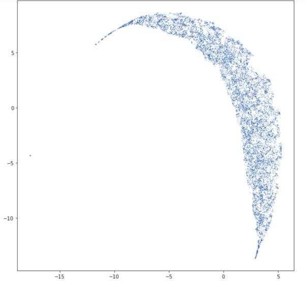
A projection of high dimensional data onto two dimensions. Made via Matplotlib.

• For histograms, play around with the parameter that controls the number of bins until you get a feel for what looks like a bin-boundary problems.
• Node-link graphs have their own special challenges, you can find more information in this illustrated essay.

A High-level Tour of Mostly Python Data-Viz

 There are a handful of capital t Truths we should all know about while living this dusty ol’ planet. Change is the only constant; “free-market efficiency” is a proposition about the flow of and perception of information and not about how well said markets work; society is basically Burning Man but with sturdier walls; we all travel towards death (not to mention tax season) at the leisurely pace of one second per second, and the quickest way to make your data visualizations look better in Python is to run the following three lines of code at the top of your Jupyter Notebook:

from Matplotlib import pyplot as plt

import Seaborn as sns

sns.set()

Once you’ve done that, you can get back to using Matplolib and contemplating the vastness of spacetime and the entire human endeavor as if nothing happened. In reality, what happened is that we’ve used the Seaborn defaults to clean up Matplotlib. (And if you don’t know, Seaborn is basically a cleaned up, higher-level version of Matplotlib, which itself is modeled on Matlab.) If Matplotlib proves too cumbersome, try Seaborn.

Let me show you the difference. First, here is some matplotlib code to visualize some data:

plt.scatter(range(len(counts)),counts)

plt.title("A Random Scatter Plot")

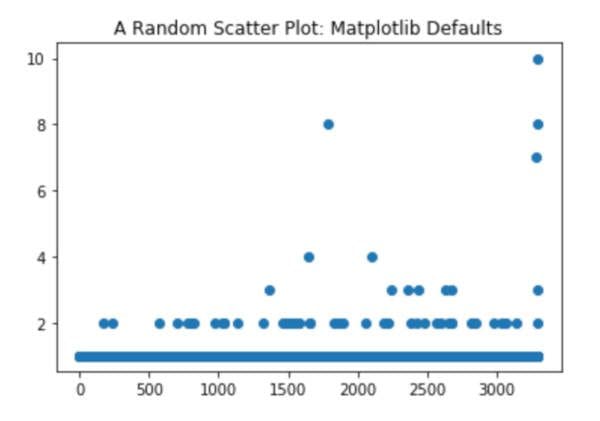
“Before”.

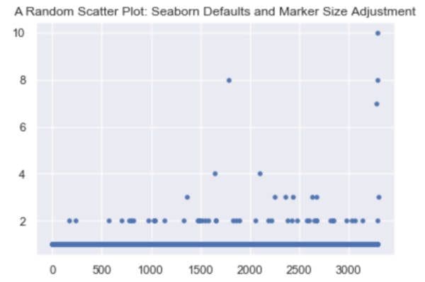
Compare this to what happens if I run the following code:

sns.set()

plt.scatter(range(len(counts)),counts,s=12)

plt.title("A Random Scatter Plot: Seaborn Defaults and Marker Size Adjustment")

Python has several packages and package-ecosystems for creating data visualizations; click here to read a detailed walkthrough. Matplotlib is the common workhorse of the bunch. While no one is going to win “designer of the year” for producing a Matplotlib illustration, it’s great for visualizing smallish datasets. At the same time, Matplotlib is neither set up for quickly visualizing 10k lines on the same plot nor for doing much that is off the beaten path.

For visualizing lots of data you might want to look at the DataShader ecosystem. Bokeh is great for interactive dashboards. For 3D, you can either use the Matplotlib extension (mplot3d), or you can check out Mayavi. And to produce great visualizations with relatively little code try Altair. Seriously, try Altair. It might just change your life.

Back in the world of R, the standard plotting libraries are ggplot2 and lattice. The former is a general-purpose plotting library, the latter makes it easy to make many small plots out of the same dataset. You can find a comprehensive list of R data visualization packages here. In looking at the basic R data visualizations, it is easy to think that.

Conclusion

Data visualization is a tool for understanding datasets. Though certain visualizations can be turned into art, the basic skills of making high-quality, day-to-day visuals are invaluable for any data-oriented person. Though you usually can’t make any grand conclusions without visualization, knowing how to manipulate, size, color, and motion of data elements is one thing we can all agree on.

Bio: SuperDataScience is an e-learning platform for data scientists who want to learn data science or improve their careers. We make the complex simple!

Related:

• Why Data Visualization Is The Most Important Skill in a Data Analyst Arsenal
• The Easy Way to Do Advanced Data Visualisation for Data Scientists
• How to choose a visualization