Master Dimensionality Reduction with these 5 Must-Know Applications of Singular Value Decomposition (SVD) in Data Science
Overview
- Singular Value Decomposition (SVD) is a common dimensionality reduction technique in data science
- We will discuss 5 must-know applications of SVD here and understand their role in data science
- We will also see three different ways of implementing SVD in Python
Introduction
“Another day has passed, and I still haven’t used y = mx + b.“
Sounds familiar? I often hear my school and college acquaintances complain that the algebra equations they spent so much time on are essentially useless in the real world.
Well – I can assure you that’s simply not true. Especially if you want to carve out a career in data science.
Linear algebra bridges the gap between theory and practical implementation of concepts. A healthy understanding of linear algebra opens doors to machine learning algorithms we thought were impossible to understand. And one such use of linear algebra is in Singular Value Decomposition (SVD) for dimensionality reduction.
You must have come across SVD a lot in data science. It’s everywhere, especially when we’re dealing with dimensionality reduction. But what is it? How does it work? And what are SVD’s applications?
I briefly mentioned SVD and its applications in my article on the Applications of Linear Algebra in Data Science. In fact, SVD is the foundation of Recommendation Systems that are at the heart of huge companies like Google, YouTube, Amazon, Facebook and many more.
We will look at five super useful applications of SVD in this article. But we won’t stop there – we will explore how we can use SVD in Python in three different ways as well.
And if you’re looking for a one-stop-shop to learn all machine learning concepts, we have put together one of the most comprehensive courses available anywhere. Make sure you check it out (and yes, SVD is in there as part of the dimensionality reduction module).
Table of contents
Applications of Singular Value Decomposition (SVD)
We are going to follow a top-down approach here and discuss the applications first. I have explained the math behind SVD after the applications for those interested in how it works underneath.
You just need to know four things to understand the applications:
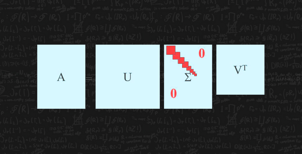
- SVD is the decomposition of a matrix A into 3 matrices – U, S, and V
- S is the diagonal matrix of singular values. Think of singular values as the importance values of different features in the matrix
- The rank of a matrix is a measure of the unique information stored in a matrix. Higher the rank, more the information
- Eigenvectors of a matrix are directions of maximum spread or variance of data
In most of the applications, the basic principle of Dimensionality Reduction is used. You want to reduce a high-rank matrix to a low-rank matrix while preserving important information.
SVD for Image Compression
How many times have we faced this issue? We love clicking images with our smartphone cameras and saving random photos off the web. And then one day – no space! Image compression helps deal with that headache.
It minimizes the size of an image in bytes to an acceptable level of quality. This means that you are able to store more images in the same disk space as compared to before.
Image compression takes advantage of the fact that only a few of the singular values obtained after SVD are large. You can trim the three matrices based on the first few singular values and obtain a compressed approximation of the original image. Some of the compressed images are nearly indistinguishable from the original by the human eye.
Here’s how you can code this in Python:
Python Code:
Output:
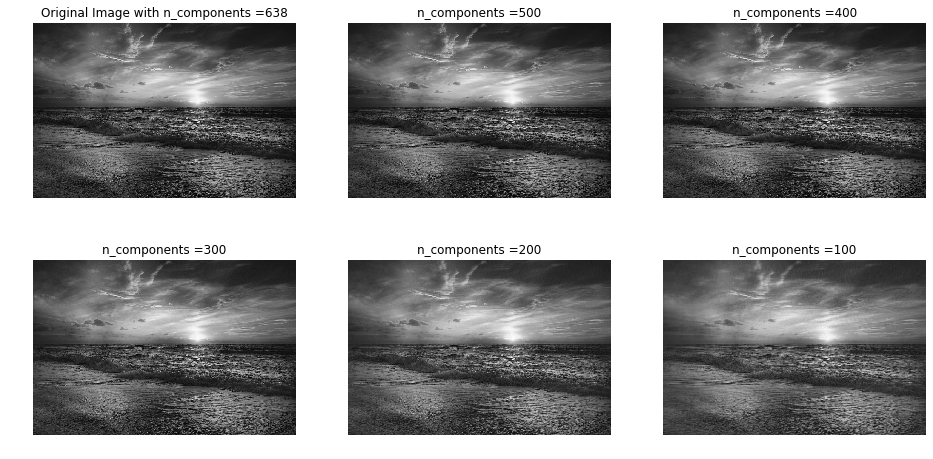
If you ask me, even the last image (with n_components = 100) is quite impressive. I would not have guessed that it was compressed if I did not have the other images for comparison.
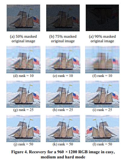
SVD for Image Recovery
Ever clicked an image in low light? Or had an old image become corrupt? We assume that we cannot get that image back anymore. It’s surely lost to the past. Well – not anymore!
We’ll understand image recovery through the concept of matrix completion (and a cool Netflix example).
Matrix Completion is the process of filling in the missing entries in a partially observed matrix. The Netflix problem is a common example of this.
Given a ratings-matrix in which each entry (i,j) represents the rating of movie j by customer i, if customer i has watched movie j and is otherwise missing, we would like to predict the remaining entries in order to make good recommendations to customers on what to watch next.
The basic fact that helps to solve this problem is that most users have a pattern in the movies they watch and in the ratings they give to these movies. So, the ratings-matrix has little unique information. This means that a low-rank matrix would be able to provide a good enough approximation for the matrix.
This is what we achieve with the help of SVD.
Where else do you see this property? Yes, in matrices of images! Since an image is contiguous, the values of most pixels depend on the pixels around them. So a low-rank matrix can be a good approximation of these images.
Here is a snapshot of the results:
Chen, Zihan. “Singular Value Decomposition and its Applications in Image Processing.” ACM, 2018
The entire formulation of the problem can be complex to comprehend and requires knowledge of other advanced concepts as well. You can read the paper that I referred to here.
SVD for Eigenfaces
The original paper Eigenfaces for Recognition came out in 1991. Before this, most of the approaches for facial recognition dealt with identifying individual features such as the eyes or the nose and developing a face model by the position, size, and relationships among these features.
The Eigenface approach sought to extract the relevant information in a face image, encode it as efficiently as possible, and compare one face encoding with a database of models encoded similarly.
The encoding is obtained by expressing each face as a linear combination of the selected eigenfaces in the new face space.
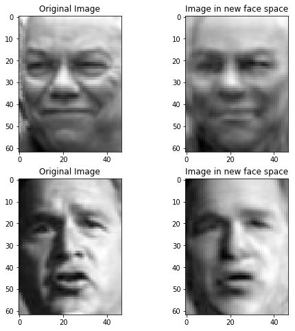
Let me break the approach down into five steps:
- Collect a training set of faces as the training set
- Find the most important features by finding the directions of maximum variance – the eigenvectors or the eigenfaces
- Choose top M eigenfaces corresponding to the highest eigenvalues. These eigenfaces now define a new face space
- Project all the data in this face space
- For a new face, project it into the new face space, find the closest face(s) in the space, and classify the face as a known or an unknown face
You can find these eigenfaces using both PCA and SVD. Here is the first of several eigenfaces I obtained after performing SVD on the Labelled Faces in the Wild dataset:
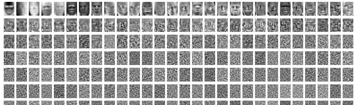
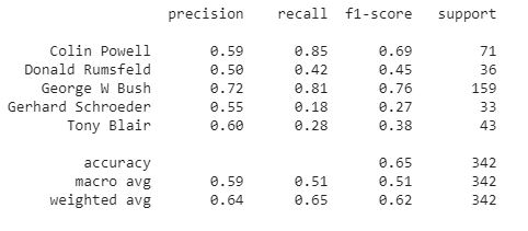
As we can see, only the images in the first few rows look like actual faces. Others look noisy and hence I discarded them. I preserved a total of 120 eigenfaces and transformed the data into the new face space. Then I used the k-nearest neighbors classifier to predict the names based on the faces.
You can see the classification report below. Clearly, there is scope for improvement. You can try adjusting the number of eigenfaces to preserve and experiment with different classifiers:
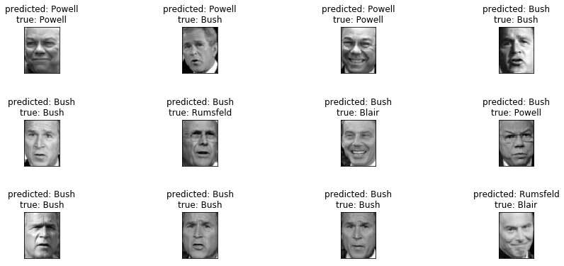
Have a look at some of the predictions and their true labels:
You can find my attempt at Facial Recognition using Eigenfaces here.
SVD for Spectral Clustering
Clustering is the task of grouping similar objects together. It is an unsupervised machine learning technique. For most of us, clustering is synonymous with K-Means Clustering – a simple but powerful algorithm. However, it is not always the most accurate.
Consider the below case:
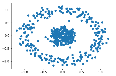
Clearly, there are 2 clusters in concentric circles. But KMeans with n_clusters = 2 gives the following clusters:
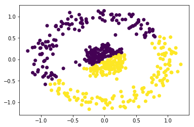
K-Means is definitely not the appropriate algorithm to use here. Spectral clustering is a technique that combats this. It has roots in Graph theory. These are the basic steps:
- Start with the Affinity matrix (A) or the Adjacency matrix of the data. This represents how similar one object is to another. In a graph, this would represent if an edge existed between the points or not
- Find the Degree matrix (D) of each object. This is a diagonal matrix with entry (i,i) equal to the number of objects object i is similar to
- Find the Laplacian (L) of the Affinity Matrix: L = A – D
- Find the highest k eigenvectors of the Laplacian Matrix depending on their eigenvalues
- Run k-means on these eigenvectors to cluster the objects into k classes
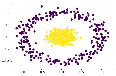
You can read about the complete algorithm and its math here. The implementation of Spectral Clustering in scikit-learn is similar to KMeans:
You will obtain the below perfectly clustered data from the above code:
SVD for Removing Background from Videos
I have always been curious how all those TV commercials and programs manage to get a cool background behind the actors. While this can be done manually, why put in that much manual effort when you have machine learning?
Think of how you would distinguish the background of a video from its foreground. The background of a video is essentially static – it does not see a lot of movement. All the movement is seen in the foreground. This is the property that we exploit to separate the background from the foreground.
Here are the steps we can follow for implementing this approach:
- Create matrix M from video – This is done by sampling image snapshots from the video at regular intervals, flattening these image matrices to arrays, and storing them as the columns of matrix M
- We get the following plot for matrix M:
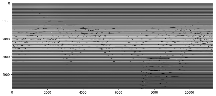
What do you think these horizontal and wavy lines represent? Take a moment to think about this.
The horizontal lines represent the pixel values that do not change throughout the video. So essentially, these represent the background in the video. The wavy lines show movement and represent the foreground.
- We can, therefore, think of M as being the sum of two matrices – one representing the background and other the foreground
- The background matrix does not see a variation in pixels and is thus redundant i.e. it does not have a lot of unique information. So, it is a low-rank matrix
- So, a low-rank approximation of M is the background matrix. We use SVD in this step
- We can obtain the foreground matrix by simply subtracting the background matrix from the matrix M
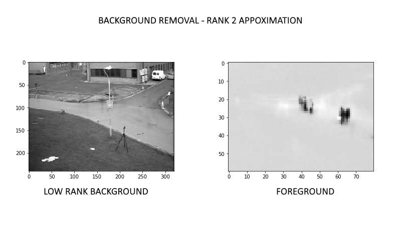
Here is a frame of the video after removing the background:
Pretty impressive, right?
We have discussed five very useful applications of SVD so far. But how does the math behind SVD actually work? And how useful is it for us as data scientists? Let’s understand these points in the next section.
What is Singular Value Decomposition (SVD)?
I have used the term rank a lot in this article. In fact, through all the literature on SVD and its applications, you will encounter the term “rank of a matrix” very frequently. So let us start by understanding what this is.
Rank of a Matrix
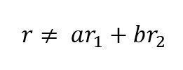
The rank of a matrix is the maximum number of linearly independent row (or column) vectors in the matrix. A vector r is said to be linearly independent of vectors r1 and r2 if it cannot be expressed as a linear combination of r1 and r2.
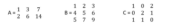
Consider the three matrices below:
- In matrix A, row r2 is a multiple of r1, r2 = 2 r1, so it has only one independent row. Rank(A) = 1
- In matrix B, row r3 is a sum of r1 and r2, r3 = r1 + r2, but r1 and r2 are independent. Rank(B) = 2
- In matrix C, all 3 rows are independent of each other. Rank(C) = 3
The rank of a matrix can be thought of as a representative of the amount of unique information represented by the matrix. Higher the rank, higher the information.
Singular Value Decomposition (SVD)
So where does SVD fit into the overall picture? SVD deals with decomposing a matrix into a product of 3 matrices as shown:
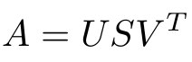
If the dimensions of A are m x n:
- U is an m x m matrix of Left Singular Vectors
- S is an m x n rectangular diagonal matrix of Singular Values arranged in decreasing order
- V is an n x n matrix of Right Singular Vectors
Why is SVD used in Dimensionality Reduction?
You might be wondering why we should go through with this seemingly painstaking decomposition. The reason can be understood by an alternate representation of the decomposition. See the figure below:
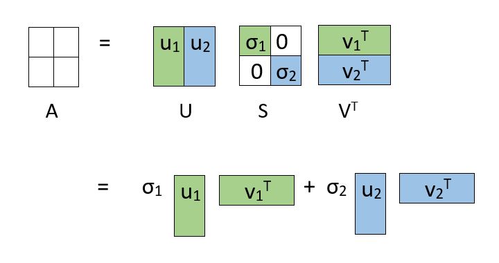
The decomposition allows us to express our original matrix as a linear combination of low-rank matrices.
In a practical application, you will observe that only the first few, say k, singular values are large. The rest of the singular values approach zero. As a result, terms except the first few can be ignored without losing much of the information. See how the matrices are truncated in the figure below:
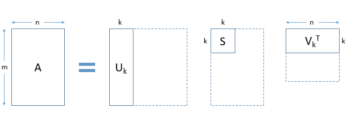
To summarize:
- Using SVD, we are able to represent our large matrix A by 3 smaller matrices U, S and V
- This is helpful in large computations
- We can obtain a k-rank approximation of A. To do this, select the first k singular values and truncate the 3 matrices accordingly
3 Ways to Perform SVD in Python
We know what SVD is, how it works, and where it is used in the real world. But how can we implement SVD on our own?
The concept of SVD sounds complex enough. You might be wondering how to find the 3 matrices U, S, and V. It is a long process if we were to calculate these by hand.
Fortunately, we do not need to perform these calculations manually. We can implement SVD in Python in three simple ways.
SVD in NumPy
NumPy is the fundamental package for Scientific Computing in Python. It has useful Linear Algebra capabilities along with other applications.
You can obtain the complete matrices U, S, and V using SVD in numpy.linalg. Note that S is a diagonal matrix which means that most of its entries are zeros. This is called a sparse matrix. To save space, S is returned as a 1D array of singular values instead of the complete 2D matrix.
Truncated SVD in scikit-learn
In most common applications, we do not want to find the complete matrices U, S and V. We saw this in dimensionality reduction and Latent Semantic Analysis, remember?
We are ultimately going to trim our matrices, so why find the complete matrices in the first place?
In such cases, it is better to use TruncatedSVD from sklearn.decomposition. You specify the number of features you want in the output as the n_components parameter. n_components should be strictly less than the number of features in the input matrix:
Randomized SVD in scikit-learn
Randomized SVD gives the same results as Truncated SVD and has a faster computation time. While Truncated SVD uses an exact solver ARPACK, Randomized SVD uses approximation techniques.
End Notes
I really feel Singular Value Decomposition is underrated. It is an important fundamental concept of Linear Algebra and its applications are so cool! Trust me, what we saw is just a fraction of SVD’s numerous uses.
I encourage you to check out this Comprehensive Guide to build Recommendation Engine from scratch to realize the power of SVD for yourself. Building this project will surely add value to your resume (and enhance your own skillset!).
Which SVD application(s) impressed you the most? Use the comments section below to let the community know.


very well explained. Very impressed by the clarity in thought and concept
Hi Sanchita, Thank you for your appreciation!
Thanks Khyati! very well explained. Can you please write a full article on discussing various SVD versions , like reduced, truncated and randomized, that would be really helpful :D.
Thank you so much, a great explanation of SVD with some terrific shared resources! I'm a little closer to understanding :)