Creating Continuous Action Bot using Deep Reinforcement Learning
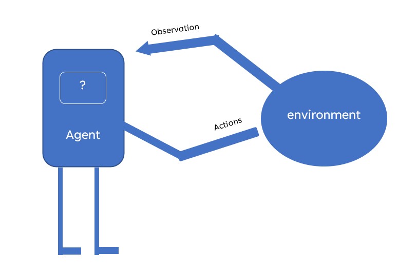
To solve any problem using reinforcement learning we need a well-defined environment that simulates our real-world problem and an agent which produces actions in the environment by taking input as observations.
Index
– Creating a custom environment using OpenAI gym
– Creating an agent using DDPG (Concept of MDP)
– Techniques to increase the performance of the model
Creating a Custom environment using OpenAI gym
Before creating our environment let’s import important libraries.
import gym
from gym import spaces
import numpy as np
Now let’s make an environment where we have a budget and we want to spend it on Facebook and Instagram advertisements. This spends will give us sales which we want to maximize. So, here is what we need to create a basic environment in python.
class OurCustomEnv(gym.Env):

    def __init__(self, sales_function, obs_range, action_range):

        self.budget = 1000                       #fixing the budget
        self.sales_function = sales_function     #calculating sales based on spends

        #we create an observation space with predefined range
        self.observation_space = spaces.Box(low = obs_range[0], high = obs_range[1],
                                                                     dtype = np.float32)

        #similar to observation, we define action space
        self.action_space = spaces.Box(low = action_range[0], high = action_range[1],
                                                                    dtype = np.float32)

     def step(self, action):

        self.budget -= np.sum(action)          #remaining budget will be old budget-sum of both spends

        reward = 0.0
        reward = self.sales_functions(action)  #gives total sales based on spends
        done = True                            #Condition for completion of episode
        info = {}

        return action, reward, done, info

    def reset(self):
        self.budget = 1000

        return np.array([0,0])
Minimal requirements to run an env is that you must have an initialization, a step function (as how the model should behave if you take some action) which will have rewards, information (any info which you need to debug or track during training, the agent does not use this) and termination status and a reset function. If our environment gets terminated then what should get reset back. You may create a seed function, to maintain reproducibility.
Creating a DDPG Agent
We will use DDPG implementation from Phil (Timothy P. Lillicrap 2015). DDPG has basic components like a replay buffer (to store all the transitions – observation state, action, reward, done, new observation state).
MDP (Markov Decision Process) requires that the agent takes the best action based on the current state. This gives step reward and a new observation state. This problem is called MDP. We store these values in a buffer called replay buffer.
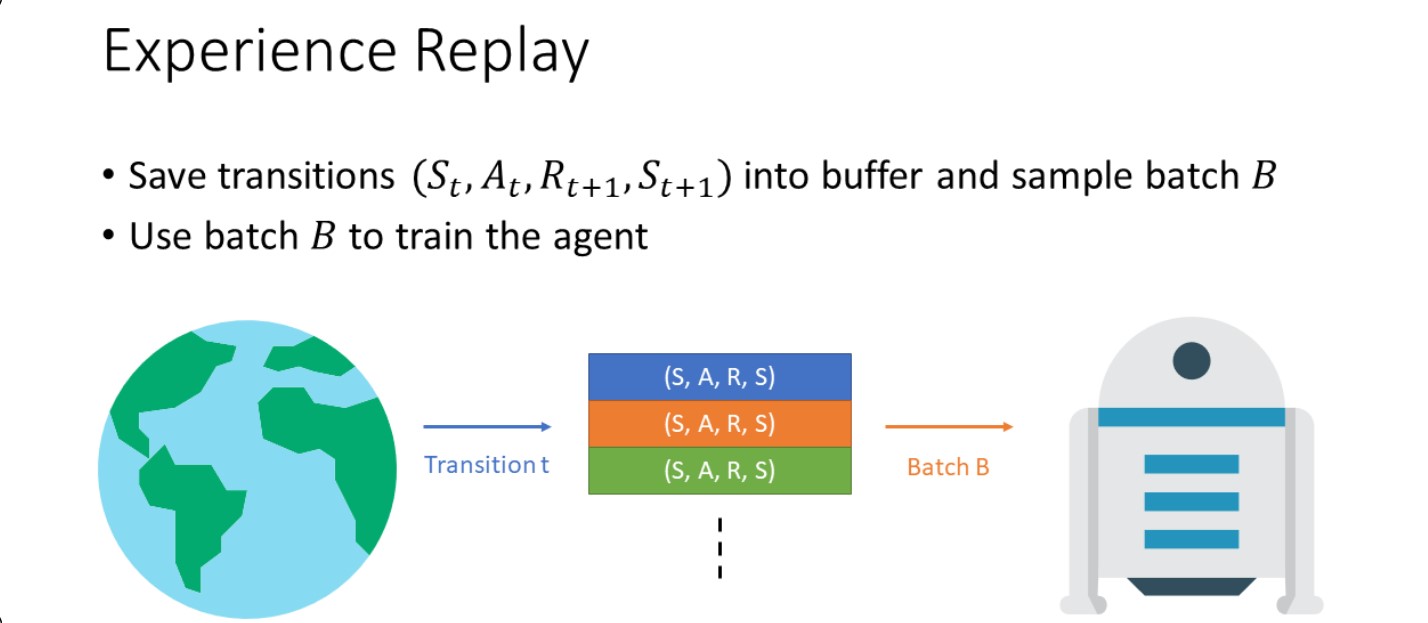
What a reply buffer does is what makes this algorithm off policy. I’ll explain off policy meaning in a bit. So, initially, our agent starts with random actions and we keep feeding it in memory until it reaches the batch size. Then from this point, the agent takes all the (states, actions, rewards, termination, new state) info from the replay buffer and learns on this. This is called an off-policy algorithm, when your agent learns based on past experiences and not from the current actions it is taking. An on-policy algorithm means it will learn on the fly, it will make a batch, learn from it and then dump that batch. So, we create our replay buffer –
Before moving on to create our Agent, Let’s import important libraries
import torch as T
import torch.nn as nn
import torch.nn.functional as F
import torch.optim as optim
Replay Buffer
class ReplayBuffer():

    def __init__(self, max_size, input_shape=2, n_actions=2):
        self.mem_size = max_size
        self.mem_cntr = 0
        self.state_memory = np.zeros((self.mem_size, input_shape))
        self.new_state_memory = np.zeros((self.mem_size, input_shape))
        self.action_memory = np.zeros((self.mem_size, n_actions))
        self.reward_memory = np.zeros(self.mem_size)
        self.terminal_memory = np.zeros(self.mem_size, dtype=np.bool)

    def store_transition(self, state, action, reward, state_, done):

        index = self.mem_cntr % self.mem_size
        self.state_memory[index] = state
        self.new_state_memory[index] = state_
        self.terminal_memory[index] = done
        self.reward_memory[index] = reward
        self.action_memory[index] = action
        self.mem_cntr += 1

    def sample_buffer(self, batch_size):
        max_mem = min(self.mem_cntr, self.mem_size)
        batch = np.random.choice(max_mem, batch_size)
        states = self.state_memory[batch]
        states_ = self.new_state_memory[batch]
        actions = self.action_memory[batch]
        rewards = self.reward_memory[batch]
        dones = self.terminal_memory[batch]

        return states, actions, rewards, states_, dones
ACTOR-CRITIC
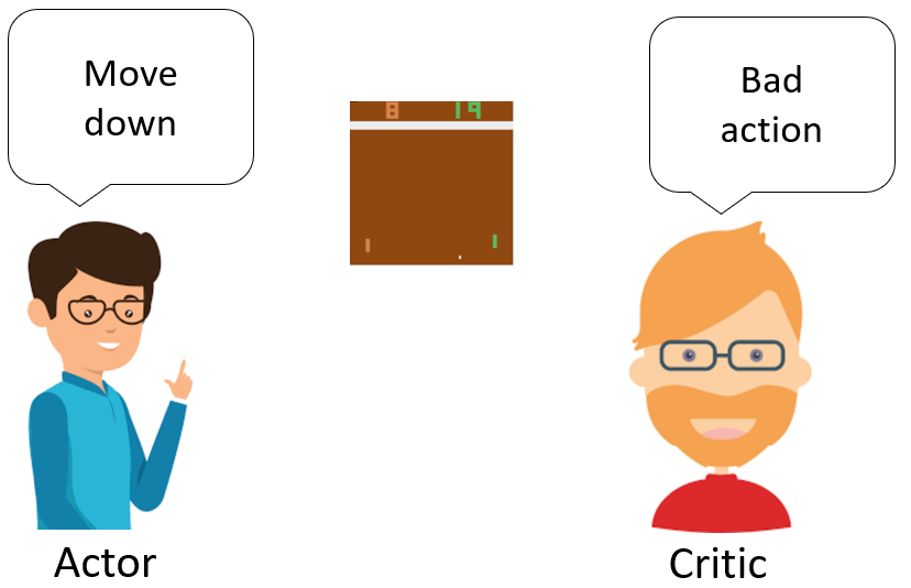
Now, we move on to the crux Actor critic method. The original paper explains quite well how it works but here is a rough idea. The actor takes a decision based on a policy, critic evaluates state-action pair and give it a Q value. If the state-action pair is good according to critics it will have a higher Q value and vice versa.
Critic Network
class CriticNetwork(nn.Module):
    def __init__(self, beta):
        super(CriticNetwork, self).__init__()
        self.input_dims = 2    #fb, insta
        self.fc1_dims = 256    #hidden layers
        self.fc2_dims = 256    #hidden layers
        self.n_actions = 2     #fb, insta
        self.fc1 = nn.Linear(2 + 2, self.fc1_dims) #state + action
        self.fc2 = nn.Linear(self.fc1_dims, self.fc2_dims)
        self.q1 = nn.Linear(self.fc2_dims, 1)
        self.optimizer = optim.Adam(self.parameters(), lr=beta)
        self.device = T.device('cuda' if T.cuda.is_available() else 'cpu')
        self.to(self.device)

    def CriticNetwork(self, state, action):
        q1_action_value = self.fc1(T.cat([state, action], dim=1 ))
        q1_action_value = F.relu(q1_action_value)
        q1_action_value = self.fc2(q1_action_value)
        q1_action_value = F.relu(q1_action_value)
        q1 = self.q1(q1_action_value)
        return q1
Now we move to actor-network, we created a similar network but here are some key points which you must remember while making the actor.
- Weight initialization is not necessary but generally, if we give it some init it learns faster.
- Choosing an optimizer is very very important, the different optimizers can make lots of differences.
- Now, how to choose the last activation function really depends on what kind of action space you are using, for example, if it is small and all values are like [-1,-2,-3] to [1,2,3] you can go ahead and tanh (squashing function), if you have [-2,-4000,-230] to [2,6000,560] you might want to change the activation function.
Actor-Network
class ActorNetwork(nn.Module):
    def __init__(self, alpha):
        super(ActorNetwork, self).__init__()
        self.input_dims = 2
        self.fc1_dims = fc1_dims
        self.fc2_dims = fc2_dims
        self.n_actions = 2
        self.fc1 = nn.Linear(self.input_dims, self.fc1_dims)
        self.fc2 = nn.Linear(self.fc1_dims, self.fc2_dims)
        self.mu = nn.Linear(self.fc2_dims, self.n_actions)
        self.optimizer = optim.Adam(self.parameters(), lr=alpha)
        self.device = T.device('cuda' if T.cuda.is_available() else 'cpu')
        self.to(self.device)

    def forward(self, state):
        prob = self.fc1(state)
        prob = F.relu(prob)
        prob = self.fc2(prob)
        prob = F.relu(prob)
        #fixing each agent between 0 and 1 and transforming each action in env
        mu = T.sigmoid(self.mu(prob))
        return mu
Note: We used 2 hidden layers since our action space was small and environment not very complex. Authors used 400 and 300 neurons for 2 hidden layers.
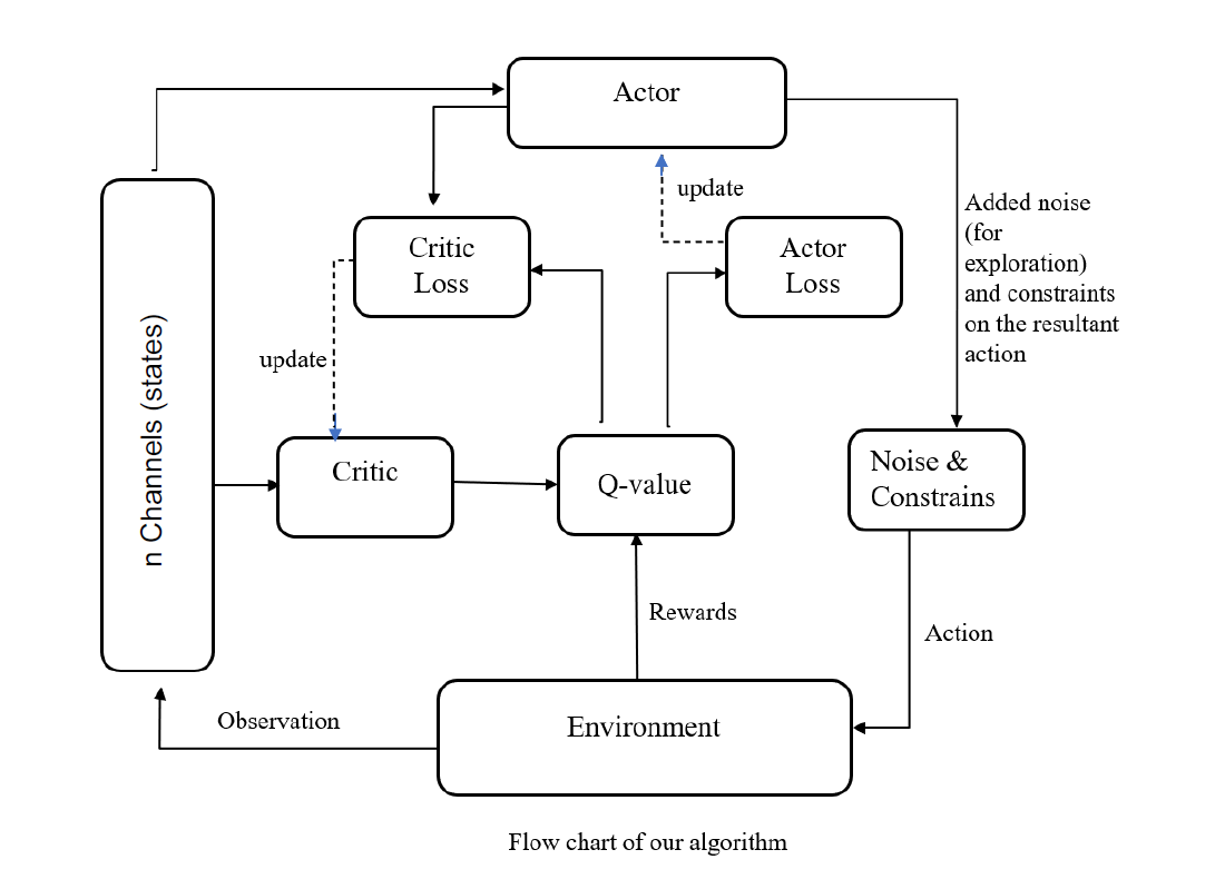
Just like gym env, the agent has some conditions too. We initialized our target networks with the same weights as our original (A-C) networks. Since we are chasing a moving target, target networks create stability and help original networks to train.
We initialize with all the requirements, as you might have noticed we have one loss function parameter too. We can use different loss functions and choose whichever works best for us (usually L1 smooth loss), paper had used mse loss, so we will go ahead and use it as default.
Here we include choosing action function, you can create an evaluation function as well, which outputs action space without noise. A remembering function (just as cover) to store it in our memory.
Update parameter function, now this is where we do soft(target networks) and hard updates(original networks). Now here it takes only one parameter Tau, this is similar to how we think a learning rate is.
It is used to soft update our target networks and in the paper, they found the best tau to be 0.001 and it usually is best across different papers (you can try and play with it).
class Agent(object):
    def __init__(self, alpha, beta, input_dims=2, tau, env, gamma=0.99,
                 n_actions=2, max_size=1000000,  batch_size=64):
        self.gamma = gamma
        self.tau = tau
        self.memory = ReplayBuffer(max_size)
        self.batch_size = batch_size
        self.actor = ActorNetwork(alpha)
        self.critic = CriticNetwork(beta)
        self.target_actor = ActorNetwork(alpha)
        self.target_critic = CriticNetwork(beta)

        self.scale = 1.0
        self.noise = np.random.normal(scale=self.scale,size=(n_actions))
        self.update_network_parameters(tau=1)

    def choose_action(self, observation):
        self.actor.eval()
        observation = T.tensor(observation, dtype=T.float).to(self.actor.device)
        mu = self.actor.forward(observation).to(self.actor.device)
        mu_prime = mu + T.tensor(self.noise(),
                                 dtype=T.float).to(self.actor.device)
        self.actor.train()
        return mu_prime.cpu().detach().numpy()

    def remember(self, state, action, reward, new_state, done):
        self.memory.store_transition(state, action, reward, new_state, done)

    def learn(self):
        if self.memory.mem_cntr < self.batch_size:
            return
        state, action, reward, new_state, done =
                                      self.memory.sample_buffer(self.batch_size)

        reward = T.tensor(reward, dtype=T.float).to(self.critic.device)
        done = T.tensor(done).to(self.critic.device)
        new_state = T.tensor(new_state, dtype=T.float).to(self.critic.device)
        action = T.tensor(action, dtype=T.float).to(self.critic.device)
        state = T.tensor(state, dtype=T.float).to(self.critic.device)

        self.target_actor.eval()
        self.target_critic.eval()
        self.critic.eval()
        target_actions = self.target_actor.forward(new_state)
        critic_value_ = self.target_critic.forward(new_state, target_actions)
        critic_value = self.critic.forward(state, action)

        target = []
        for j in range(self.batch_size):
            target.append(reward[j] + self.gamma*critic_value_[j]*done[j])
        target = T.tensor(target).to(self.critic.device)
        target = target.view(self.batch_size, 1)

        self.critic.train()
        self.critic.optimizer.zero_grad()
        critic_loss = F.mse_loss(target, critic_value)
        critic_loss.backward()
        self.critic.optimizer.step()

        self.critic.eval()
        self.actor.optimizer.zero_grad()
        mu = self.actor.forward(state)
        self.actor.train()
        actor_loss = -self.critic.forward(state, mu)
        actor_loss = T.mean(actor_loss)
        actor_loss.backward()
        self.actor.optimizer.step()

        self.update_network_parameters()

    def update_network_parameters(self, tau=None):
        if tau is None:
            tau = self.tau

        actor_params = self.actor.named_parameters()
        critic_params = self.critic.named_parameters()
        target_actor_params = self.target_actor.named_parameters()
        target_critic_params = self.target_critic.named_parameters()

        critic_state_dict = dict(critic_params)
        actor_state_dict = dict(actor_params)
        target_critic_dict = dict(target_critic_params)
        target_actor_dict = dict(target_actor_params)

        for name in critic_state_dict:
            critic_state_dict[name] = tau*critic_state_dict[name].clone() +
                                      (1-tau)*target_critic_dict[name].clone()

        self.target_critic.load_state_dict(critic_state_dict)

        for name in actor_state_dict:
            actor_state_dict[name] = tau*actor_state_dict[name].clone() +
                                      (1-tau)*target_actor_dict[name].clone()
        self.target_actor.load_state_dict(actor_state_dict)
The most crucial part is the learning function. First, we feed the network with samples until it reaches batch size and then start sampling from batches to update our networks. Calculate critic and actor losses. Then just soft update all the parameters.

env = OurCustomEnv(sales_function, obs_range, act_range)

agent = Agent(alpha=0.000025, beta=0.00025, tau=0.001, env=env,
              batch_size=64, n_actions=2)

score_history = []
for i in range(10000):
    obs = env.reset()
    done = False
    score = 0
    while not done:
        act = agent.choose_action(obs)
        new_state, reward, done, info = env.step(act)
        agent.remember(obs, act, reward, new_state, int(done))
        agent.learn()
        score += reward
        obs = new_state

    score_history.append(score)
Results
Just in few minutes, we have training results ready. Agent exhausts almost full budget and we have a graph during training –
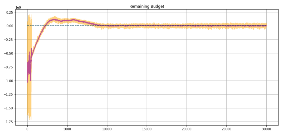
These results can be achieved even faster if we make changes in hyperparameters and reward functions.
Also thanks to Phil and Andrej Karpathy for their marvellous work.
The media shown in this article are not owned by Analytics Vidhya and are used at the Author’s discretion.
Student of IIT Roorkee '22. Upcoming Data Scientist at Yum! (parent of KFC, Taco Bells, Pizza Hut). Skilled in Research as well as experienced in working with complex mathematical models for real-world applications. Pursuing Quant as a hobby.


Very good post. I want to reproduce but I do not find the sales_function function. I the entire code available?
sales function is missing would like to be able to run the example to learn about ddpg and custum gym env
Hi Nihal, Thanks for this example of continuous action RL. The env() object requires some object definitions that have not been provided and hence the code does not execute. It might help to provide a default sales_function, and ranges for observations and actions to get the code running.
Hi Nihal, Thanks for this example of continuous action RL. The env() object requires some object definitions that have not been provided and hence the code does not execute. It might help to provide a default sales_function, and ranges for observations and actions to get the code running.