Creating Linear Model, It’s Equation and Visualization for Analysis
This article was published as a part of the Data Science Blogathon.
Introduction
Have you ever been tasked with visualizing the relationship between each feature and the target in a Linear regression model to analyze the line of best fit? Well, soon or later you’ll have to. This article explains this in easy to understand steps. Let’s go!
Linear Regression:
.png)
Fig. 1.0: The Basic Linear Regression model Visualization
The Linear model (Linear Regression) was probably the first model you learned and created, using the model to predict the Target’s continuous values. You sure must have been happy that you’ve completed a model. You were probably also taught the theories behind its functionality– The Empirical Risks Minimization, The Mean Squared Loss, The Gradient descent, The Learning Rate among others.
Well, this is great and all of a sudden I was called to explain a model I created to the manager, all those terms were like jargons to him, and when he asked for the model visualization (as in fig 1.0) that is the model fit hyperplane(the red line) and the data points(the blue dots). I froze to my toes not knowing how to create that in python code.
Well, That’s what the first part of this article is about Creating the Basic Linear Model Visualization in your Jupyter notebook in Python.
Let’s begin using this random data:
| X | y |
| 1 | 2 |
| 2 | 3 |
| 3 | 11 |
| 4 | 13 |
| 5 | 28 |
| 6 | 32 |
| 7 | 50 |
| 8 | 59 |
| 9 | 85 |
Method 1: Manual Formulation
Importing our library and creating the Dataframe:
now at this stage, there are two ways to perform this visualization:
1.) Using Mathematical knowledge
2.) Using the Linear_regression Attribute for scikit learns Linear_model.
- Let’s get started with the Math😥😥.
just follow through it’s not that difficult, First we define the equation for a linear relationship between y(dependent variables/target) and X(independent variable/features) as :
y = mX + c
where y = Target
X = features
a = slope
b = y-intercept constant
To create the model’s equation we have to get the value of m and c , we can get this from the Y and X with the equations below:
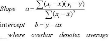
The slope, a is interpreted as the product between the summation of the difference between each individual x value and its mean and the summation of the difference between each individual y point and its mean then divided by the summation of the square of each individual x and its mean.
The intercept is simply the mean of y minus the product of the slope and mean of x
That is a lot to take in. probably read it over and over till you get it, try reading with the picture
👆👆 that was the only challenge; if you’ve understood it congratulations let’s move on.
Now writing this in python code is ‘eazy-pizzy’ using the numpy library, check it out👇👇.
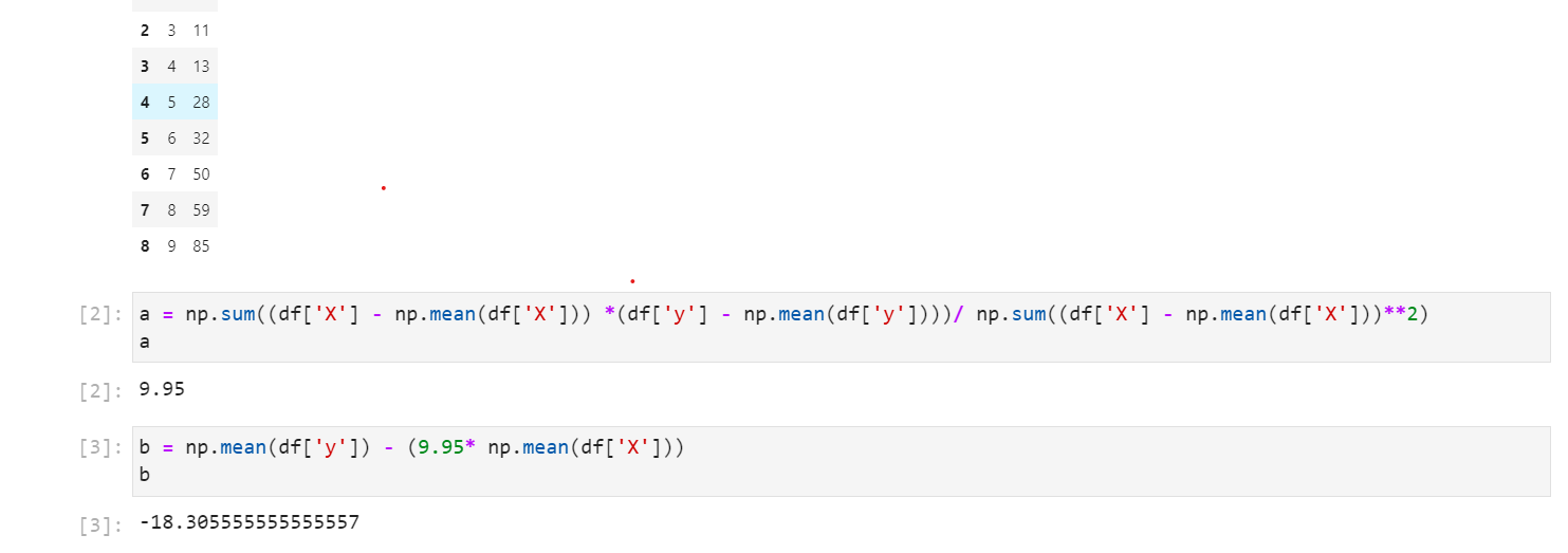
now we have our a and b we just insert it to the equation—-> y = 9.95 -1218.56x
To blow your mind now, did you know that this is the model’s equation. and we just created a model without using scikit learn. we will confirm it now using the second method which is the scikit learn Linear Regression package
Method 2: Using scikit-learn’s Linear regression
We’ll be importing Linear regression from scikit learn, fit the data on the model then confirming the slope and the intercept. The steps are in the image below.
so you can see that there is almost no difference, now let us visualize this as in fig 1.
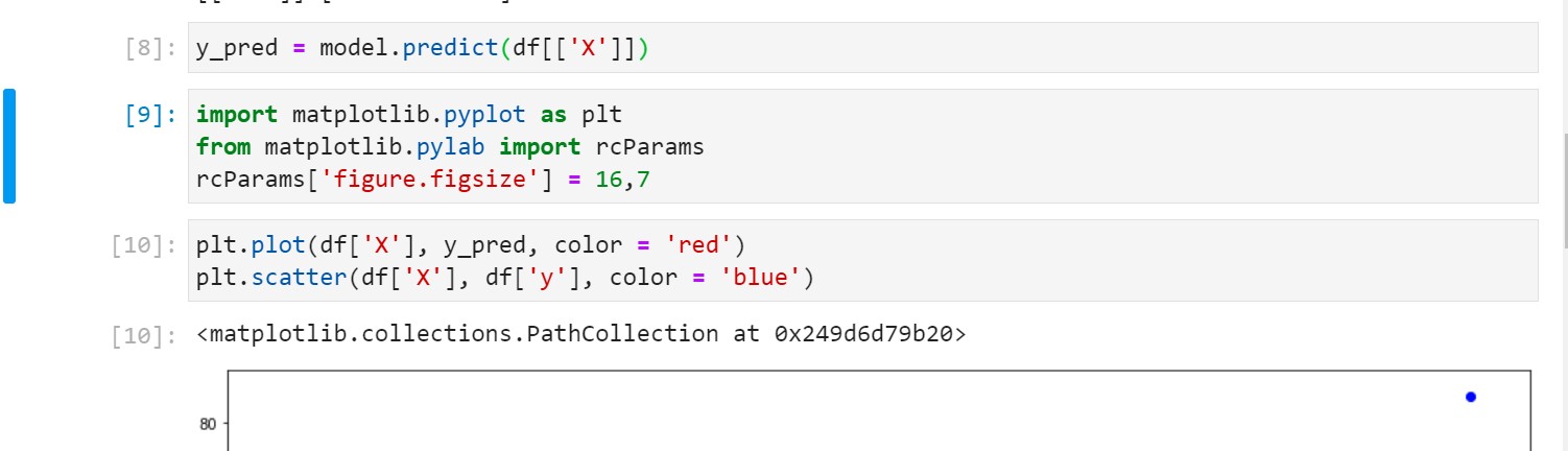
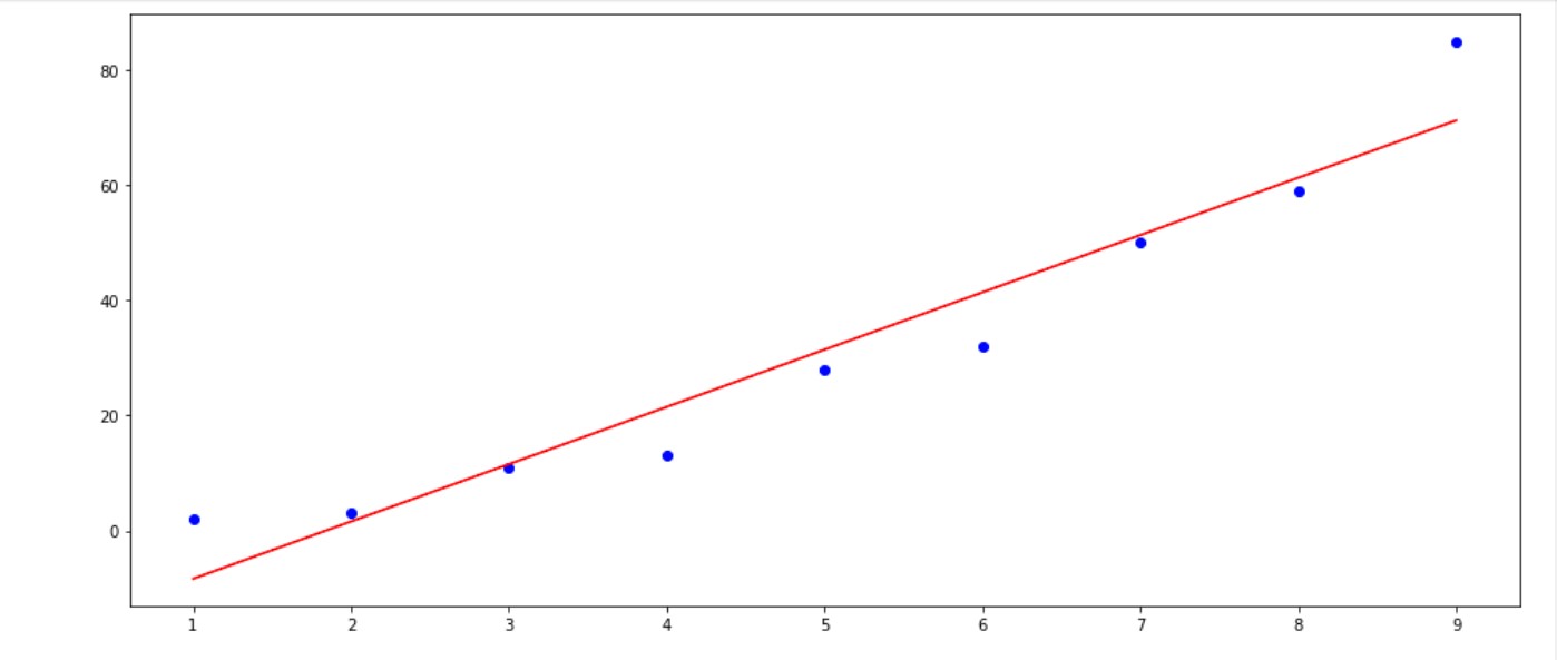
The red line is our line of best fit that will be used for the prediction and the blue point are our initial data. With this, I had something to report back to the manager. I particularly did this for each feature with the target to add more insight.
Now we have achieved our goal of creating a model and showing its plotted graph
This technique may be time-consuming when it comes to data with larger sizes and should only be used when visualizing your line of best fit with a particular feature for analysis purposes. It is not really necessary during modeling unless requested, Errors and calculation may suck up your time and computation resources especially if you’re working with 3D and higher data. But the insight gotten is worth it.
I hope you enjoyed the article if yes that great, you can also tell me how to improve in any way. I still have a lot to share especially on regressions(Linear, Logistics, and Polynomial ).
Thank You for reading through.


