H2O Framework for Machine Learning
This article is an overview of H2O, a scalable and fast open-source platform for machine learning. We will apply it to perform classification tasks.

H2O is a scalable and fast open-source platform for machine learning. We will apply it to perform classification tasks. The dataset we are using is the Bank Marketing Dataset. Here we need to train a model which will be able to predict if the client of the bank opens the term deposit on the basis of his/her personal features of the client, marketing campaign features and current macroeconomic conditions.
During the model creation we explore various core components and functions from the H2O toolkit. You should understand that while this article covers some basic concepts of H2O, if you need more detailed information you should go to the H2O website and read documentation.
Note: for installation instructions please use the official website.
Preparation
We need to import needed libraries first:
import pandas as pd
import numpy as np
import h2o
pd.set_option('display.width', 5000)
The first thing you should do is to start the H2O. You can run method h2o.init() to initialize H2O. Many different parameters can be given to h2o.init() method in order to set up the H2O according to your needs. So, here you can change some global settings of the H2O. Nevertheless, in most cases it is enough to call this methods without any parameters, like we did below:
h2o.init()

You can see that the output from this method consists of some meta-information about your H2O cluster.
The next thing we should do is to import the dataset we will work with. This is the .csv file and the H2O has function upload_file() which will load the dataset in the memory. It is worth to say that the H2O can work with several data sources (both local and remote) and support different file formats.
bank_df = h2o.upload_file("bank-additional-full.csv")
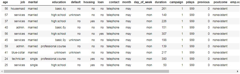
To take a look at the dataset, you can simply type in its name and run the cell. The top 10 rows are displayed by default.
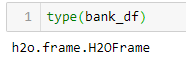
Looking at the type of this variable, we can see that the type is h2o.frame.H2OFrame. So, this is not a pandas object, but the own object of the H2O.
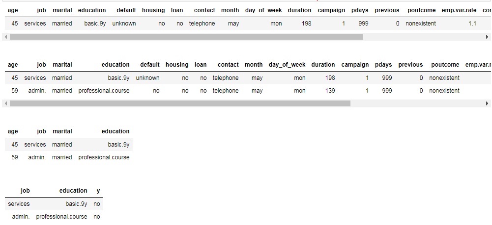
However, you can index and slice this H2OFrame in a familiar manner:
# show 6th row
print(bank_df[5,:])
# show 6-7 rows
print(bank_df[5:7,:])
# show first 4 columns from 6-7 rows
print(bank_df[5:7,0:4])
# show job,education and y columns from 6-7 rows
print(bank_df[5:7, ['job', 'education', 'y']])
You can check the shape of the H2OFrame by accessing .shape attribute of it. Also, some useful information (type of columns, min, average, max values, standard deviation, number of zeros, missing values) can be generated by .describe() method.


As we can see, there are no missing data in our dataset. We have 20 columns with different categorical, integer and real number features and 1 target column (y). The target variable is binary and can take values "yes" if the customer want to subscribe a term deposit or "no" if not.
In the next cell we extract the names of columns into the variable x. Then, we remove the name of the target column (y) from this list. Also, we write the name of the target variable in the variable y.
x = bank_df.names
x.remove("y")
print(x)
Y = "y"

The first model
Now let's train certain model. First, we need to split our dataset into training and testing parts. H2O allows to do this by using function split_frame(). If you pass only one element in the list as the first argument (or argument ratios), this element defines the fraction of the training dataset. The rest is the testing set. If you pass two elements, the first means training, the second - testing, and the rest - validation set. Here we want to take 70% of the sample as training set and 30% as testing set. We also fix the random state to get the reproducible results.
train, test = bank_df.split_frame([0.7], seed=42)
For the beginning, we want to use Random Forest model to classify data points. The H2ORandomForestEstimator can be found in the module h2o.estimators.
from h2o.estimators import H2ORandomForestEstimator
Then we create an instance of the estimator. Here you can specify many different parameters. We set the number of trees to 200 by assigning 200 to ntrees parameter. After this, we call the method train on the instance of estimator. We should pass names of columns with features into variable x and the name of the target column into variable y. Also, we specify training and validation samples. After we run this cell, we can see the progress bar below it, reflecting the status of the training process.
rf = H2ORandomForestEstimator(ntrees=200)
rf.train(x=x,
         y=y,
         training_frame=train,
         validation_frame=test)

The model details can be accessed by looking at the instance of the estimator:

A lot of interesting and useful information is available here. You can notice two blocks of information. The first one is reported on the train set and the second is about test set. There are different model performance metrics (MSE, RMSE, LogLoss, AUC, Gini etc.). Confusion matrix is a very interesting metric for error analysis. H2O allows to look at confusion matrices both on the train and test set. The total fraction of errors as well as for each label are also displayed in the confusion matrices.
Interesting table is about maximum metrics at their respective errors. In the binary classification, model returns the probability of the instance to have the positive class. And then this probability should be compared with some threshold to decide if this is the positive class or negative. H2O shows in this table the maximum values for different metrics and also specify the thresholds used when achieving this maximum metrics. For example, in our case we can achieve the perfect precision on the test set by choosing the threshold 0.985. The maximum accuracy on the test set is 0.911 and it can be achieved when you choose 0.5294 as the threshold. The highest F1-score corresponds to the threshold 0.331.
While implementing your model in solution you can choose the threshold which is the best suitable for your needs. Also, you can try some more advanced things, like choosing the threshold by combining thresholds reported for max values of different metrics for both train and test sets.
One more interesting table here is the table with feature importances. The most informative columns are scaled_importance and percentage. You can see that the duration feature has the maximum predictive power for this task and dataset. This feature means the duration of a phone call with a client. Top 5 other important features, besides duration are macroeconomic indicators euribor3m and nr.employed, and also age and job of the client.
Now we want to manually compute the accuracy on the test set.
In the next cell we make predictions. You can see that method predict() returns a dataframe with the answer (yes or no) in the first column and the probabilities for no and yes in the next two columns.
rf = H2ORandomForestEstimator(ntrees=200)
rf.train(x=x,
         y=y,
         training_frame=train,
         validation_frame=test

In the next cell we count the number of cases where the predictions equals to the actual answers and then we compute the mean which will be the accuracy of the prediction. We can see that the accuracy is 0.9041 or around 90.4%. If you return back and look at the confusion matrix you can notice that if you subtract the total error for the test set (0.0958) from 1, you will get ~0.9041, which is the accuracy we found manually.
(predictions["predict"] == test["y"]).mean()
Other algorithms
H2O provides several different models for training. Let's try some of them.
The first algorithm we want to train using the neural network. To use this model we need to import H2ODeepLearningEstimator from h2o.estimators.deeplearning module. Then, we need to create an instance of this estimator. Like in the previous example with Random Forest, here you can pass many different parameters to control the model and training process. It is important to set up the architecture of the neural network. In the parameter hidden we pass a list with a number of neurons in hidden layers. So, this parameter controls both the number of hidden layers and neurons in these layers. We set up 3 hidden layers with 100, 10 and 4 neurons in each respectively. Also, we set the activation function to be Tanh.
from h2o.estimators.deeplearning import H2ODeepLearningEstimator
dl = H2ODeepLearningEstimator(hidden=[100, 10, 4],activation='Tanh')
dl.train(x=x, y=y, training_frame=train, validation_frame=test)
predictions_dl = dl.predict(test)
print((predictions_dl["predict"] == test["y"]).mean())

We can see that the accuracy is slightly lower than with Random Forest. Maybe we can fine-tune the model's parameters to get better performance.
In the next few cells we train linear model. Binomial family means that we want to perform classification with logistic regression. lambda_search allows searching optimal regularization parameter lambda.
from h2o.estimators.glm import H2OGeneralizedLinearEstimator
lm = H2OGeneralizedLinearEstimator(family="binomial",
                                   lambda_search=True)
lm.train(x=x,
         y=y,
         training_frame=train,
         validation_frame=test)
predictions_lm = lm.predict(test)
print((predictions_lm["predict"] == test["y"]).mean())

The last model we want to use here is the Gradient Boosting algorithm. With the default parameters it can give the best results amongst all other algorithms
from h2o.estimators.gbm import H2OGradientBoostingEstimator
gb = H2OGradientBoostingEstimator()
gb.train(x=x,
         y=y,
         training_frame=train,
         validation_frame=test)

predictions_gb = gb.predict(test)
print((predictions_gb["predict"] == test["y"]).mean())

It is worth to mention about XGBoost integration in the H2O platform. XGBoost is one of the most powerful algorithms which implements the gradient boosting idea. You can install it standalone, but it is also very convenient to use XGBoost in H2O. In the cell below you can see how to create an instance of H2OXGBoostEstimator and how to train it. You should understand that XGBoost uses many parameters and very often can be very sensitive to the changes in these parameters.
param = {
         "ntrees" : 400,
         "max_depth" : 4,
         "learn_rate" : 0.01,
         "sample_rate" : 0.4,
         "col_sample_rate_per_tree" : 0.8,
         "min_rows" : 5,
         "seed": 4241,
         "score_tree_interval": 100
         }
predictions_xgb = xgb.predict(test)
print((predictions_xgb["predict"] == test["y"]).mean())

There are several other models available in the H2O. You should see documentation if you want to know more.
Cross validation in H2O
Cross validation is one of the core techniques used in machine learning. The basic idea is to split the dataset into several parts (folds) and then train the model on all except one fold, which will be used later for testing. On this, the current iteration finishes and the next iteration begins. On the next iteration, the testing fold is included in the training sample. Instead, certain fold from the previous training set is used for testing.
For example, we split the dataset into 3 folds. On first iteration we use 1st and 2nd folds for training and 3rd for testing. On the second iteration 1st and 3rd folds are used for training and 2nd for testing. On the third iteration the 1st folds is used for testing and the 2nd and 3rd are used for training.
Cross validation allows to estimate the model's performance in a more accurate and reliable way.
In H2O it is simple to do cross validation. If the model supports it, there is an optional parameter nfolds which can be passed when creating an instance of the model. You should specify the number of folds for cross validation using this parameter.
H2O builds nfolds + 1 models. An additional model is trained on all the available data. This is the main model you will get as the result of training.
Let's train Random Forest and perform cross validation with 3 folds. Note that we are not passing the validation (test) set, but the entire dataset.
rf_cv = H2ORandomForestEstimator(ntrees=200, nfolds=3)
rf_cv.train(x=x, y=y, training_frame=bank_df)

If you look at the output in the cell above, you will notice some differences.
The first is that instead of reporting on validation data the model reports on cross-validation data.
The second is that there is a table with cross-validation metrics summary. Here you can see many different metrics, their values for each of the fold as the test fold, the mean of these values and the standard deviation for each of the metric. For example, for first fold we get accuracy 0.9006, for second - 0.904, for third - 0.903. The mean of these values is 0.9025 and the standard deviation is 0.001. You should understand that it is important not only to have "good" values for metrics, but also to have low standard deviation. This means that your model behaves well on different examples in the dataset. But the interpretation of the results of the cross-validation isn't actually the goal of this article, so let's move to the next chapter!
Model tuning using GridSearch
Often, you need to try many different parameters and their combinations to find one which produces the best performance of the model. It is hard and sometimes tedious to do everything by hand. Grid search allows to automate this process. All you need to do is to specify the set of hyperparameters you want to try and run the GridSearch instance. The system will try all possible combinations of the parameters (train and test models for each combination). Let's look how this tool can be used in H2O.
First, you need to import the instance of the GridSearch object:
from h2o.grid.grid_search import H2OGridSearch
Now you need to specify all possible parameters which you want to try. We are going to search for an optimal combination of parameters for the XGBoost model we have built earlier. The parameters are placed inside a python dictionary where the keys are the names of the parameters and the values are the lists with possible values of these parameters.
xgb_parameters = {'max_depth': [3, 6],
                  'sample_rate': [0.4, 0.7],
                  'col_sample_rate': [0.8, 1.0],
                  'ntrees': [200, 300]}
The next step is a creation of the GridSearch instance. You should pass a model, id of the grid, and the dictionary with hyperparameters.
xgb_grid_search = H2OGridSearch(model=H2OXGBoostEstimator,
                                grid_id='example_grid',
                                hyper_params=xgb_parameters)
Eventually, you can run the grid search. Note that we set the higher learning rate, because grid search is a very time-consuming process. The number of models to train grows rapidly with the growth of number of hyperparameters. So, taking into account that this is only a learning example, we don't want to test many hyperparameters.
xgb_grid_search.train(x=x,
                      y=y,
                      training_frame=train,
                      validation_frame=test,
                      learn_rate=0.3,
                      seed=42)
We can get the results of the grid search by using method get_grid() of the GridSearch instance. We want to sort the results by accuracy metric in the descending order.
grid_results = xgb_grid_search.get_grid(sort_by='accuracy',
                                        decreasing=True)
print(grid_results)
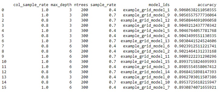
You can see that the highest accuracy is obtained by using combination of 1.0 column sample rate, 0.4 sample rate, 200 trees and the maximum depth of one tree equal to 3.
AutoML
H2O provides the ability to perform automated machine learning. The process is very simple and is oriented on the users without much knowledge and experience in machine learning. AutoML will iterate through different models and parameters trying to find the best. There are several parameters to specify, but in most cases all you need to do is to set only the maximum runtime in seconds or maximum number of models. You can think about AutoML as something similar to GridSearch but on the level of models rather than on the level of parameters.
from h2o.automl import H2OAutoML
autoML = H2OAutoML(max_runtime_secs=120)
autoML.train(x=x,
             y=y,
             training_frame=bank_df)
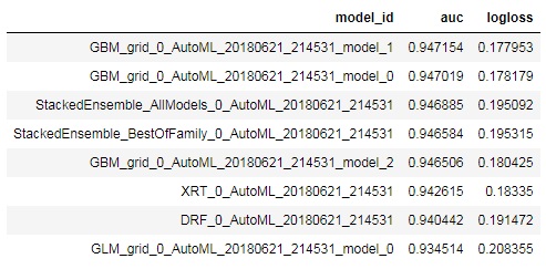
We can take a look on the table with all tried models and their corresponding performance by checking the .leaderboard attribute of the autoML instance. GBM with 0.94 AUC metric seems to be the best model here.
leaderboard = autoML.leaderboard
print(leaderboard)
Take a look at the best model:

You can predict on the test set directly from the autoML instance.
predictionAML = autoML.predict(test)
Conclusion
This article is just a brief introductory overview of the H2O functionality. This is a great machine learning platform that can make some areas of machine learning work of engineers work more simple. It is a continuously developing framework. In the same way, in our opinion, it cannot be used alone. Instead, other instruments used along with H2O can make the machine learning process faster and more convenient.
In this article, we covered some basic data manipulation operations in H2O, looked at several machine learning models provided by H2O, learned how to perform cross-validation and grid search, became familiar with the automated machine learning in H2O.
You should understand that there are some features of the H2O which are below the scope of this article. So, if you are interested in learning more, please, read the official documentation.
ActiveWizards is a team of data scientists and engineers, focused exclusively on data projects (big data, data science, machine learning, data visualizations). Areas of core expertise include data science (research, machine learning algorithms, visualizations and engineering), data visualizations ( d3.js, Tableau and other), big data engineering (Hadoop, Spark, Kafka, Cassandra, HBase, MongoDB and other), and data intensive web applications development (RESTful APIs, Flask, Django, Meteor).
Original. Reposted with permission.
Related:
- Automated Machine Learning: How do teams work together on an AutoML project?
- Automated Machine Learning Project Implementation Complexities
- Comparison of Top 6 Python NLP Libraries