Feature Scaling Techniques in Python – A Complete Guide
This article was published as a part of the Data Science Blogathon.
Introduction
In Data Processing, we try to change the data in such a way that the model can process it without any problems. And Feature Scaling is one such process in which we transform the data into a better version. Feature Scaling is done to normalize the features in the dataset into a finite range.
I will be discussing why this is required and what are the common feature scaling techniques used.
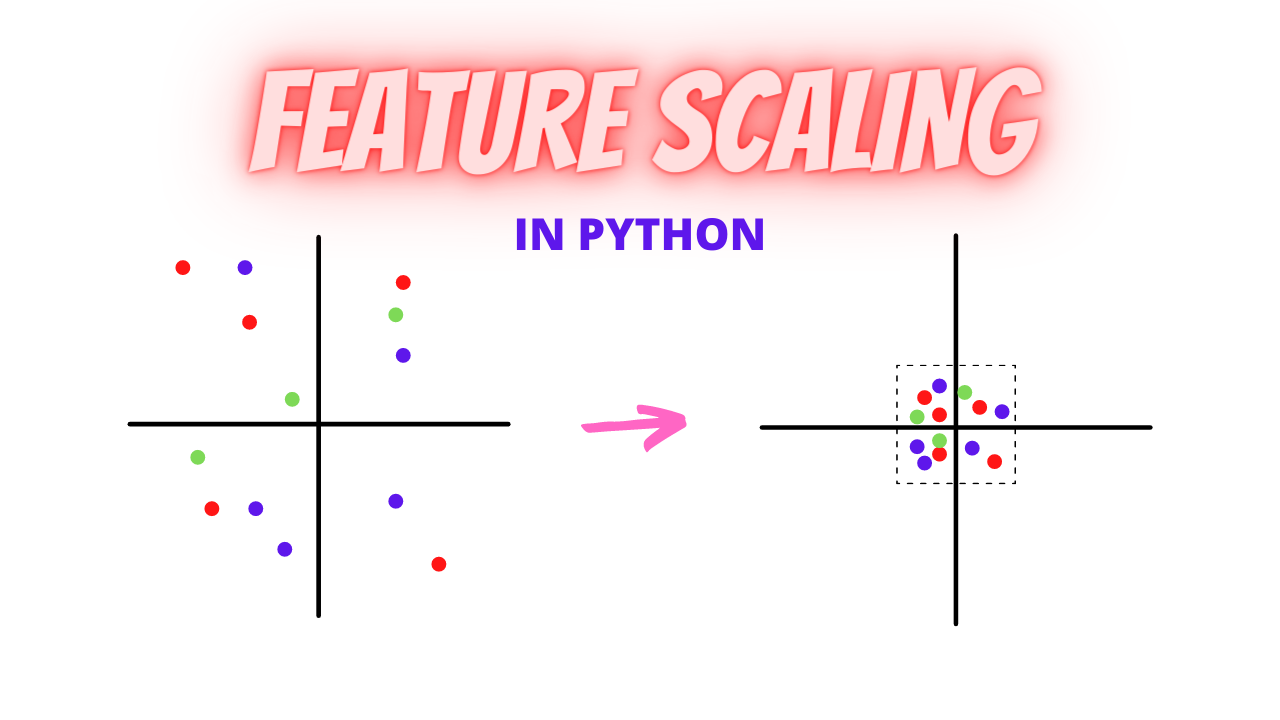
Table Of Contents
- Why Feature Scaling is Important?
- Absolute Maximum Scaling
- Min-Max Scaling
- Normalization
- Standardization
- Robust Scaling
- Is Feature Scaling actually helpful?
Why Feature Scaling?
Real Life Datasets have many features with a wide range of values like for example let’s consider the house price prediction dataset. It will have many features like no. of. bedrooms, square feet area of the house, etc.
As you can guess, the no. of bedrooms will vary between 1 and 5, but the square feet area will range from 500-2000. This is a huge difference in the range of both features.
Many machine learning algorithms that are using Euclidean distance as a metric to calculate the similarities will fail to give a reasonable recognition to the smaller feature, in this case, the number of bedrooms, which in the real case can turn out to be an actually important metric.
Eg: Linear Regression, Logistic Regression, KNN
There are several ways to do feature scaling. I will be discussing the top 5 of the most commonly used feature scaling techniques.
- Absolute Maximum Scaling
- Min-Max Scaling
- Normalization
- Standardization
- Robust Scaling
Absolute Maximum Scaling
- Find the absolute maximum value of the feature in the dataset
- Divide all the values in the column by that maximum value
If we do this for all the numerical columns, then all their values will lie between -1 and 1. The main disadvantage is that the technique is sensitive to outliers. Like consider the feature *square feet*, if 99% of the houses have square feet area of less than 1000, and even if just 1 house has a square feet area of 20,000, then all those other house values will be scaled down to less than 0.05.
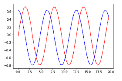
I will be working with the sine and cosine functions throughout the article and show you how the scaling techniques affect their magnitude. sin() will be ranging between -1 and +1, and 50*cos() will be ranging between -50 and +50.
This is how they actually look, you will not even be able to see that the red one is a sine graph, it basically looks like a straight squiggly line when compared to the big blue graph.
y1_new = y1/max(y1)
y2_new = y2/max(y2)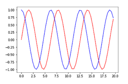
See from the graph that now both the datasets are ranging from -1 to +1 after the scaling.
This might become significantly small with many data points below even 0.01 even if there is a single big outlier.
Min Max Scaling
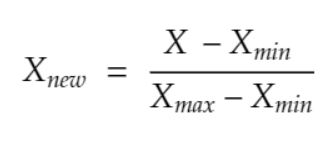
In min-max you will subtract the minimum value in the dataset with all the values and then divide this by the range of the dataset(maximum-minimum). In this case, your dataset will lie between 0 and 1 in all cases whereas in the previous case, it was between -1 and +1. Again, this technique is also prone to outliers.
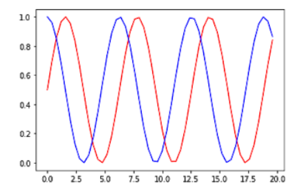
y1_new = (y1-min(y1))/(max(y1)-min(y1))
y2_new = (y2-min(y2))/(max(y2)-min(y2))
plt.plot(x,y1_new,'red')
plt.plot(x,y2_new,'blue')
[<matplotlib.lines.Line2D at 0x7f6e1bf8fd30>]
Normalization
Instead of using the min() value in the previous case, in this case, we will be using the average() value.
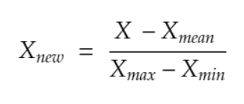
In scaling, you are changing the range of your data while in normalization you arere changing the shape of the distribution of your data.
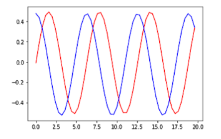
y1_new = (y1-np.mean(y1))/(max(y1)-min(y1))
y2_new = (y2-np.mean(y2))/(max(y2)-min(y2))
plt.plot(x,y1_new,'red')
plt.plot(x,y2_new,'blue')
[<matplotlib.lines.Line2D at 0x7f6e1bfb5518>]
Standardization
In standardization, we calculate the z-value for each of the data points and replaces those with these values.
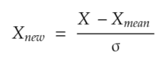
This will make sure that all the features are centred around the mean value with a standard deviation value of 1. This is the best to use if your feature is normally distributed like salary or age.
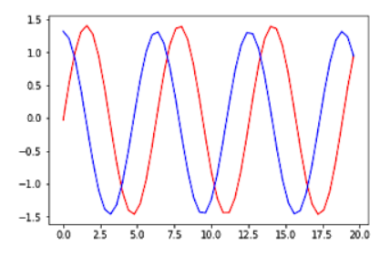
y1_new = (y1-np.mean(y1))/np.std(y1)
y2_new = (y2-np.mean(y2))/np.std(y2)
plt.plot(x,y1_new,'red')
plt.plot(x,y2_new,'blue')
[<matplotlib.lines.Line2D at 0x7f6e25e66e10>]
Robust Scaling
In this method, you need to subtract all the data points with the median value and then divide it by the Inter Quartile Range(IQR) value.
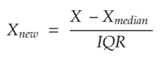
IQR is the distance between the 25th percentile point and the 50th percentile point.
This method centres the median value at zero and this method is robust to outliers.
from scipy import stats
IQR1 = stats.iqr(y1, interpolation = 'midpoint')
y1_new = (y1-np.median(y1))/IQR1
IQR2 = stats.iqr(y2, interpolation = 'midpoint')
y2_new = (y2-np.median(y2))/IQR2
plt.plot(x,y1_new,'red')
plt.plot(x,y2_new,'blue')
[<matplotlib.lines.Line2D at 0x7f6e25e19080>]
Is Feature Scaling actually helpful?
Let’s look at an example of a College Admission dataset, in which your goal is to predict the chance of admission for each student based on the other features given.
You can download the dataset from the link below.
https://www.kaggle.com/mohansacharya/graduate-admissions
import pandas as pd
df = pd.read_csv("Admission_Predict.csv")
df.head()
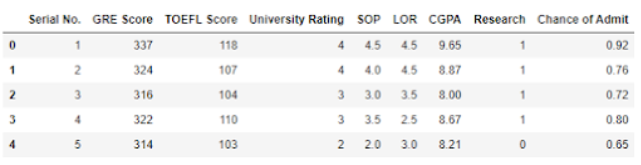
The dataset has a wide variety of features with different ranges. The first column Serial No. is not important, so I am going to be deleting it. Then I am splitting the dataset into training and test dataset.
df.drop("Serial No.",axis=1,inplace=True)
y = df['Chance of Admit ']
df.drop("Chance of Admit ",axis=1,inplace=True)
from sklearn.model_selection import train_test_split
x_train,x_test,y_train,y_test = train_test_split(df,y,test_size=0.2)
I am going to be building a linear regression model, first without normalization, and next with normalization, let’s check whether there is any improvement in the accuracy.
from sklearn.linear_model import LinearRegression
lr = LinearRegression()
lr.fit(x_train,y_train)
pred = lr.predict(x_test)
from sklearn import metrics
rmse = np.sqrt(metrics.mean_squared_error(y_test,pred))
rmse
0.06845052747026953
See that without normalization the root mean squared error value comes out to be 0.0684, as most of the values in the `y` are less than 0.5.
from sklearn.preprocessing import StandardScaler
sc = StandardScaler()
sc.fit(df)
df = sc.transform(df)
from sklearn.model_selection import train_test_split
x_train,x_test,y_train,y_test = train_test_split(df,y,test_size=0.2)
from sklearn.linear_model import LinearRegression
lr = LinearRegression()
lr.fit(x_train,y_train)
pred = lr.predict(x_test)
from sklearn import metrics
rmse = np.sqrt(metrics.mean_squared_error(y_test,pred))
rmse
0.05674870151306346
See that, we are able to get a significant reduction in the error when we used the standardization technique.
Thanks for reading the article.
The media shown in this article are not owned by Analytics Vidhya and is used at the Author’s discretion.


