Application of Machine Learning in Medical Domain!
This article was published as a part of the Data Science Blogathon
Introduction
While doing any Machine Learning Project, the utmost thing is Pipeline that includes mainly the following components:
- Data Preprocessing,
- Exploratory Data Analysis,
- Feature Engineering,
- Model Building and Evaluation, etc.
Therefore, for Machine Learning Engineers and Data Scientists aspirants, it becomes very important to understand the Machine Learning Pipeline.
Let’s understand the motivation behind all these concepts:
After a better idea about the pipeline, we can implement any of the Machine Learning Project which gives better clarity about our project.
So, In this article, we will be discussing the complete Machine learning pipeline with the help of a machine learning project of Medical Dataset.

Image Source: Google Images
Problem statement
- We will build a Linear regression model for the Medical cost dataset.
- The dataset contains age, sex, BMI(body mass
index), children, smokers, and region feature, as independent variables, and charge as a dependent variable. - We will predict individual medical costs billed
by health insurance.
Definition & Working Principle
- Linear Regression is Supervised learning the algorithm used when the target/dependent
the variable is continuous in real numbers. - It finds a relationship between the dependent variable y and one or more independent variable
x using the best fit line. - It works on the principle of Ordinary Least Square(OLS) or Means squared Error (MSE).
- In Statistics, OLS is a method to estimate unknown parameters of the linear regression function, its goal is to minimize the sum of square differences between observed dependent
variables in the given data set and those predicted by the linear regression algorithm.
Step-1: Import Necessary Dependencies
In this step, we will import the necessary dependencies of Python such as:
- Matrix Manipulation: Numpy
- Data Manipulation: Pandas
- Data Visualization: Matplotlib
- Advanced-Data Visualization: Seaborn
import pandas  as pd
import numpy as np
import matplotlib.pyplot as plt
import seaborn as sns
plt.rcParams['figure.figsize'] = [8,5]
plt.rcParams['font.size'] =14
plt.rcParams['font.weight']= 'bold'
plt.style.use('seaborn-whitegrid')
Step-2: Read and Load the Dataset
Now, we will read and load the dataset using Pandas.
2.1: Load the Dataset
df = pd.read_csv('insurance.csv')
2.2: Number of rows and columns in the dataset
print('nNumber of rows and columns in the data set: ',{'Rows':df.shape[0], 'columns':df.shape[1]})
Output:
Number of rows and columns in the data set: {'Rows': 1338, 'columns': 7}
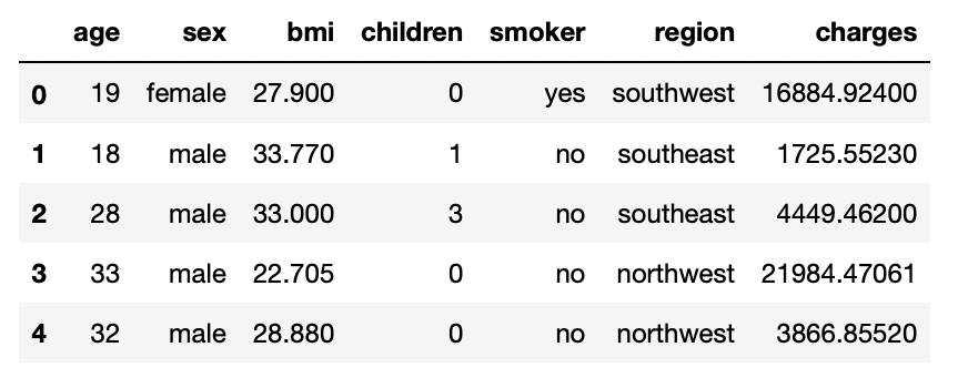
2.3: Print the first five rows of the dataset
df.head()
Output:
Step-3: Exploratory Data Analysis
In this step, we will explore the data and try to find some insights by visualizing the data properly, by using the Pandas and Seaborn library functions.
3.1: Check for duplicated data
duplicate=df.duplicated()
print(duplicate.sum())
Output:
1
3.2: Remove the duplicated records
df.drop_duplicates(inplace=True)
3.3: Now verify if there is any duplicated record left or not
dp1=df.duplicated()
print(dp1.sum())
Output:
0
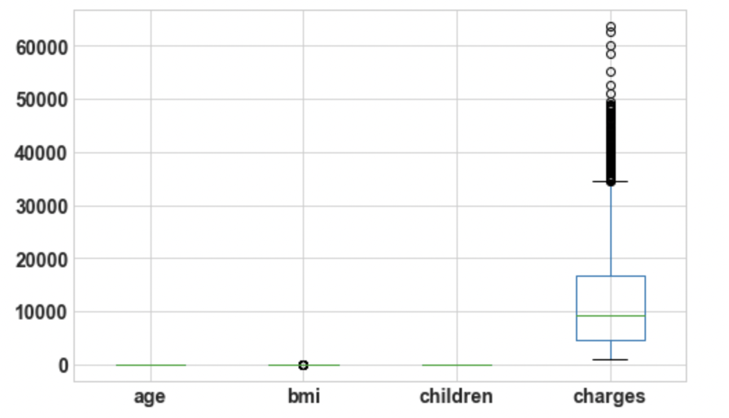
3.4: Draw boxplot for Outlier Analysis
df.boxplot();
Output:
3.5: Size of the DataFrame
print("No of elements in the dataframe is",df.size)
Output:
No of elements in the dataframe is 9359
3.6: Print data Types of all columns
print(df.dtypes)
Output:
3.7: Draw the pairplot for complete Dataset
sns.pairplot(df);
3.8: Visualize the distribution of data for every feature(For plotting histogram)
import matplotlib.pyplot as plt
df.hist(bins=50, figsize=(20, 15));
Output:
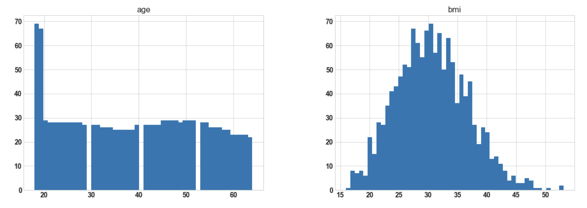
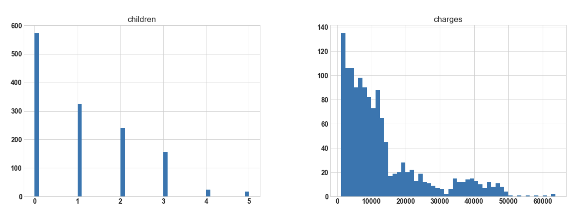
Conclusion: Hereafter plotting the histogram for numerical columns, we observe that ‘bmi’ is almost
normally distributed whereas ‘charges’ are most probably to be right-skewed.
3.9: Memory Usage by each of the columns
df.memory_usage()
Output:
Index       10696
age         10696
sex         10696
bmi         10696
children    10696
smoker      10696
region      10696
charges     10696
dtype: int64
3.10: Print Index of the DataFrame
df.index
Output:
Int64Index([   0,    1,    2,    3,    4,    5,    6,    7,    8,    9,
            ...
            1328, 1329, 1330, 1331, 1332, 1333, 1334, 1335, 1336, 1337],
           dtype='int64', length=1337)
3.11: Print number of unique values per columns
df.nunique()
Output:
age           47
sex            2
bmi          548
children       6
smoker         2
region         4
charges     1337
dtype: int64
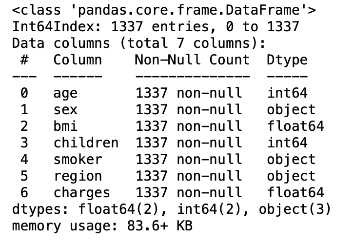
3.12: Brief information about the dataset( coincise information about the data frame)
df.info()
Output:
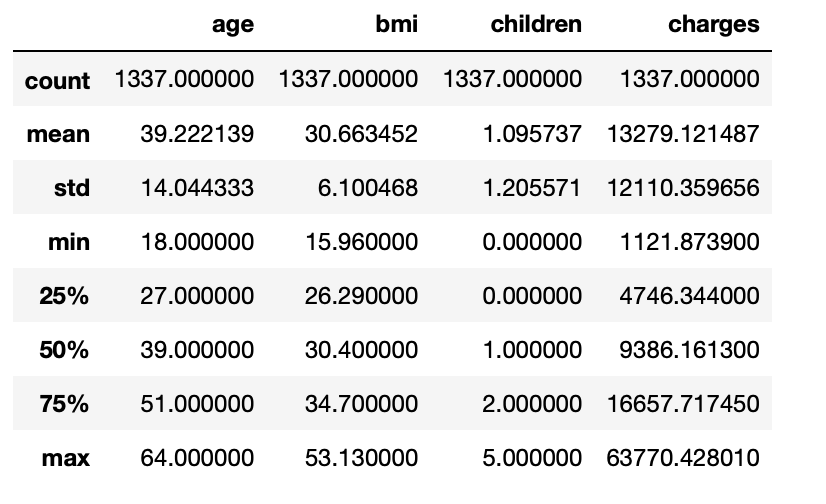
3.13: Statistical measure of all the numerical columns
df.describe()
Output:
3.14: Print name of all columns present in the dataset
df.columns
Output:
Index(['age', 'sex', 'bmi', 'children', 'smoker', 'region', 'charges'], dtype='object')
3.15: Name for all numerical columns
num_cols=[col for col in df.columns if df[col].dtypes!='O']
num_cols
Output:
['age', 'bmi', 'children', 'charges']
3.16: Name for all categorical columns
cat_cols=[col for col in df.columns if df[col].dtypes=='O']
cat_cols
Output:
['sex', 'smoker', 'region']
3.17: Print unique values for categorical columns
print(df['sex'].unique())
print(df['smoker'].unique())
print(df['region'].unique())
Output:
['female' 'male']
['yes' 'no']
['southwest' 'southeast' 'northwest' 'northeast']
3.18: Finding the sum of missing values per column if present
df.isnull().sum()
Output:
age         0
sex         0
bmi         0
children    0
smoker      0
region      0
charges     0
dtype: int64
3.19: Plotting of heatmap to visualize missing values
plt.figure(figsize=(12,4))
sns.heatmap(df.isnull(),cbar=False,cmap='viridis',yticklabels=False)
plt.title('Missing value in the dataset');
Output:
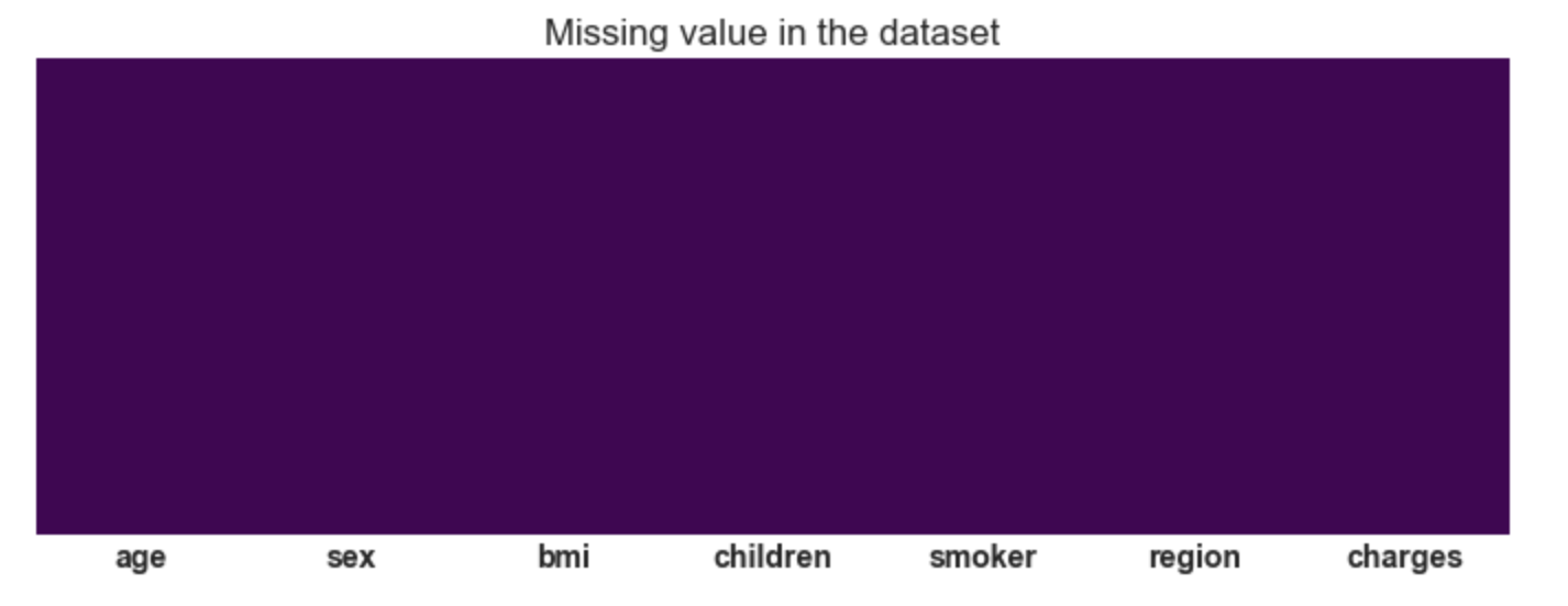
Conclusion: There are no missing values in
the dataset.
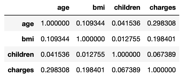
3.20: Correlation values b/w numerical columns
corr_mat=df.corr()
corr_mat
Output:
3.21: Correlation of dependent column wrt independent columns
corr_mat['charges'].sort_values(ascending=False)
Output:
charges     1.000000
age         0.298308
bmi         0.198401
children    0.067389
Name: charges, dtype: float64
3.22: Correlation plot
sns.heatmap(df.corr(),annot= True);
Output:
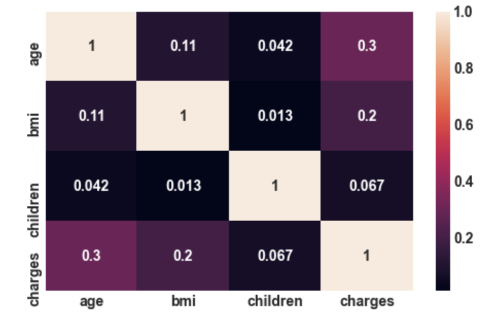
Conclusion: There is not that much correlation
between independent features. So, here we do
not have the problem of multicollinearity.
3.23: Plot the distribution of the dependent variable
import warnings
warnings.filterwarnings('ignore')
f= plt.figure(figsize=(12,4))
ax=f.add_subplot(121)
sns.distplot(df['charges'],bins=50,color='y',ax=ax)
ax.set_title('Distribution of insurance charges')
ax=f.add_subplot(122)
sns.distplot(np.log10(df['charges']),bins=40,color='b',ax=ax)
ax.set_title('Distribution of insurance charges in $log$ scale')
ax.set_xscale('log');
Output:
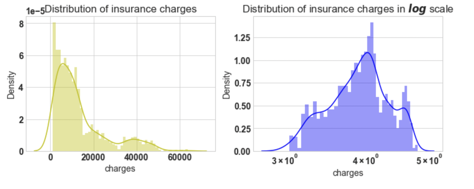
Conclusion: If we look at the first plot the charges vary
from 1120 to 63500, the plot is right-skewed. And In the second plot, we will apply a natural log,
then the plot approximately tends to normal. For further analysis, we will apply log on target variable charges.
Step-4: Data Preprocessing
Machine learning algorithms are not able to work directly with categorical data so we have to convert categorical data into numbers. There are mainly three techniques to do this i.e.,
- Label Encoding: Label encoding refers to transforming the word labels into numerical
form so that the algorithms can understand how to operate on them. - One hot encoding: It represents the categorical variables in the form of binary vectors. It allows the representation of categorical data to be more expressive. Firstly, the categorical values have been mapped to integer values, which is known as label encoding. Then, each integer value is represented as a binary vector that is all zero values except for the index of the integer, which is marked with a1
- Dummy variable trap: This is a scenario when the independent variables are collinear with each other.
Here in this problem, we use a dummy variable trap. By using the pandas get_dummies function we can do
all the above three steps in the line of code. We will this function to get dummy variables for sex,
children, smoker, region features. By setting drop_first =True function will remove dummy variables traps by dropping one variable and the original variable.
4.1: Apply the pd.get_dummies() function
df_encode = pd.get_dummies(data = df, prefix = 'OHE', prefix_sep='_', columns = cat_cols, drop_first =True, dtype='int8')
4.2 Let’s verify the dummy variable process
print('Columns in original data frame:n',df.columns.values)
print('nNumber of rows and columns in the dataset:',df.shape)
print('nColumns in data frame after encoding dummy variable:n',df_encode.columns.values)
print('nNumber of rows and columns in the dataset:',df_encode.shape)
Output:
Columns in original data frame:
 ['age' 'sex' 'bmi' 'children' 'smoker' 'region' 'charges']
Number of rows and columns in the dataset: (1337, 7)
Columns in data frame after encoding dummy variable:
 ['age' 'bmi' 'children' 'charges' 'OHE_male' 'OHE_yes' 'OHE_northwest'
 'OHE_southeast' 'OHE_southwest']
Number of rows and columns in the dataset: (1337, 9)
Box-Cox transformation :
- It is a technique to transform non-normal dependent variables into a normal distribution.
- Most of the time, Normality becomes a crucial assumption for many statistical techniques; so if your data is not normal, then applying a Box-Cox implies that you can run a broader number of tests.
- All that we need to perform this transformation is to find the lambda value and apply the rule shown below to your variable. The trick of Box-Cox transformation is to find lambda value, however, in practice, this is quite affordable.
4.3: Log transform of the dependent variable
from scipy.stats import boxcox
y_bc,lam, ci= boxcox(df_encode['charges'],alpha=0.05)
ci,lam
Output:
((-0.011576269777122257, 0.09872104960017168), 0.043516942579678274)
4.4: Log transform
df_encode['charges'] = np.log(df_encode['charges'])
Step-5: Splitting of Data into Training and Test Subset
Here we use the train_test_split() function
with parameters as dependent and independent
variables with test_ratio=0.3 from
model_selection module.
from sklearn.model_selection import train_test_split
# Independent variables(predictor)
X = df_encode.drop('charges',axis=1)
# dependent variable(response)
y = df_encode['charges']
# Now, split the data
X_train, X_test, y_train, y_test = train_test_split(X,y,test_size=0.3,random_state=23)
Step-6: Model Building
6.1: add x0 =1 to dataset
X_train_0 = np.c_[np.ones((X_train.shape[0],1)),X_train]
X_test_0 = np.c_[np.ones((X_test.shape[0],1)),X_test]
# Step2: build model
theta = np.matmul(np.linalg.inv( np.matmul(X_train_0.T,X_train_0) ), np.matmul(X_train_0.T,y_train))
# The parameters for linear regression model
parameter = ['theta_'+str(i) for i in range(X_train_0.shape[1])]
columns = ['intersect:x_0=1'] + list(X.columns.values)
parameter_df = pd.DataFrame({'Parameter':parameter,'Columns':columns,'theta':theta})
6.2: Scikit Learn module( # Note: x0 =1 is no need to add, sklearn will take care of it.)
from sklearn.linear_model import LinearRegression
lin_reg = LinearRegression(fit_intercept=True,normalize=False)
lin_reg.fit(X_train,y_train)
#Parameter
sk_theta = [lin_reg.intercept_]+list(lin_reg.coef_)
parameter_df = parameter_df.join(pd.Series(sk_theta, name='Sklearn_theta'))
parameter_df
Output:
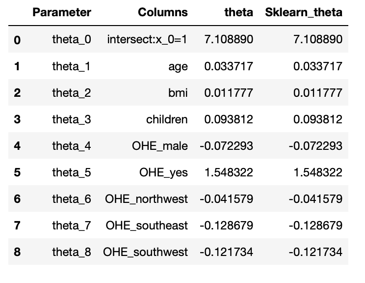
Conclusion: The parameters obtained from both models are the same. So we successfully build our model
using normal equations and verified using the sklearn linear regression module.
Step-7: Model Evaluation
7.1: Normal equation
y_pred_norm =  np.matmul(X_test_0,theta)
#Evaluation: MSE
J_mse = np.sum((y_pred_norm - y_test)**2)/ X_test_0.shape[0]
# R_square calculation
sse = np.sum((y_pred_norm - y_test)**2)
sst = np.sum((y_test - y_test.mean())**2)
R_square = 1 - (sse/sst)
7.2: sklearn regression module
y_pred_sk = lin_reg.predict(X_test)
#Evaluation: MSE
from sklearn.metrics import mean_squared_error
J_mse_sk = mean_squared_error(y_pred_sk, y_test)
# R_square
R_square_sk = lin_reg.score(X_test,y_test)
Step-8: Predictions on Test Dataset
8.1: Prediction of test data using the normal equation
print(y_pred_norm)
print(y_pred_sk)
Step-9: Finding Evaluation Metrics
9.1: Mean Squared Error for Model using Normal Equation
print('The Mean Square Error(MSE) or J(theta) is: ',J_mse)
Output:
The Mean Square Error(MSE) or J(theta) is: 0.19026739560428377
9.2: R-Squared for Model using the Normal Equation
print('The R_2 score by using the normal equation is: ',R_square)
Output:
The R_2 score by using the normal equation is: 0.785908962562808
9.3: Mean Squared Error for Model using Sklearn Library
print('The Mean Square Error(MSE) or J(theta) is: ',J_mse_sk)
Output:
The Mean Square Error(MSE) or J(theta) is: 0.19026739560428194
9.4: R-Squared for Model using Sklearn Library
print('The R_2 score by using the sklearn library is: ',R_square_sk)
Output:
The R_2 score by using the sklearn library is: 0.78590896256281
Conclusion: Since our sklearn model and normal equation are giving almost the same value of R2 and Mean
squared error, these two models are very closely related and the test predictions of both the models
are very close to each other.
Step-10: Model Validation
To validate the model we need to check a
few assumptions of the linear regression model. The common assumption for the Linear Regression model
are as follows:
- Linear Relationship: In linear regression the relationship between the dependent and independent
variable to be linear. This can be checked by scattering plotting between Actual value Vs Predicted value. - The residual error plot should be normally distributed.
- The mean of residual error should be 0 or close to 0 as much as possible.
- Linear regression requires all variables to be multivariate normal. This assumption can best be
checked with a Q-Q plot. - Linear regression assumes that there is little or no Multicollinearity in the data. Multicollinearity happens when the independent variables are correlated with each other. To identify the correlation between independent variables and the strength of that correlation, we use Variance Inflation Factor(VIF).
- VIF=1/1-R2: If VIF >1 & VIF <5 moderate correlation, VIF < 5 critical level of multicollinearity.
- Homoscedasticity: The data are homoscedastic meaning the residuals are equal across the regression
line. We can look at residual Vs fitted value scatter plots. The heteroscedastic plot would exhibit a funnel
shape pattern.
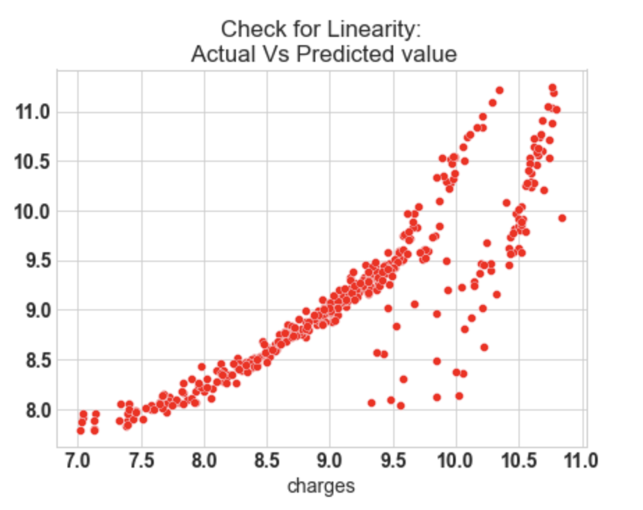
10.1: Check for Linearity
f = plt.figure(figsize=(15,5))
ax = f.add_subplot(121)
sns.scatterplot(y_test,y_pred_sk,ax=ax,color='r')
ax.set_title('Check for Linearity:n Actual Vs Predicted value')
Output:
10.2: Check for Residual normality & mean
ax = f.add_subplot(122)
sns.distplot((y_test - y_pred_sk),ax=ax,color='b')
ax.axvline((y_test - y_pred_sk).mean(),color='k',linestyle='--')
ax.set_title('Check for Residual normality & mean: n Residual eror');
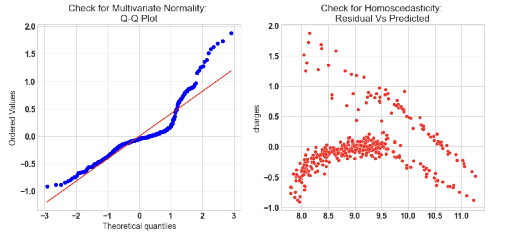
10.3: Check for Multivariate Normality
# Quantile-Quantile plot
f,ax = plt.subplots(1,2,figsize=(14,6))
import scipy as sp
_,(_,_,r)= sp.stats.probplot((y_test - y_pred_sk),fit=True,plot=ax[0])
ax[0].set_title('Check for Multivariate Normality: nQ-Q Plot')
#Check for Homoscedasticity
sns.scatterplot(y = (y_test - y_pred_sk), x= y_pred_sk, ax = ax[1],color='r')
ax[1].set_title('Check for Homoscedasticity: nResidual Vs Predicted');
Output:
10.4: Check for Multicollinearity
#Variance Inflation Factor
VIF = 1/(1- R_square_sk)
VIF
Output:
4.670910150983689
Conclusion:
The model assumption linear regression as follows:
- In our model, the actual vs predicted plot is curved so the linear assumption fails.
- The residual mean is zero and the residual error plot is right-skewed.
- Q-Q plot shows as the value log value greater than 1.5 trends to increase.
- The plot exhibits heteroscedastic error and will increase after a certain point.
- Variance inflation factor value is less than 5, so no multicollinearity.
End Notes
I hope you enjoyed the article.
If you want to connect with me, please feel free to contact me on Email
Your suggestions and doubts are welcomed here in the comment section. Thank you for reading my article!
The media shown in this article are not owned by Analytics Vidhya and are used at the Author’s discretion.


