Juicing out the Diabetes Patterns amongst Indians using Machine Learning
This article was published as a part of the Data Science Blogathon
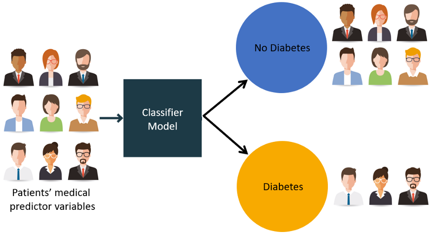
Image Source: Google Image
India is considered to be the diabetes capital of the world. Diabetes is one of the primary causes of mortality in India. There are diagnostic tools available in the forms of Random Blood Sugar test, Fasting and PP (Post Prandial) Sugar test, and HbA1C test which is a glycated hemoglobin test. Though these reliable tests are available for years, it becomes very important to spot the disease early as many people might develop it silently especially in the young workforce. In this regard, Machine Learning may play a stellar role in preventing diabetes among those who are at moderate to high risk by carefully predicting patterns based upon several variables. In this article, we would look into the biological aspects of diabetes, after that, we would analyze the dataset, then how machine learning would help, and finally, with the help of the PIMA Indian diabetes dataset, we would look into the patterns of data to fulfill our objective.
What is Diabetes?
There are 2 types of diabetes viz. insulin-dependent diabetes mellitus (IDDM)/Type-I diabetes and non-insulin-dependent diabetes mellitus (NIDDM)/Type-II diabetes. Type-I is a disorder of carbohydrate metabolism due to insufficient insulin secretion which could be hereditary or acquired. Type-II diabetes is a condition in which the sensitivity of body cells to insulin gets reduced.
Symptoms of diabetes and risks associated with untreated diabetes
The typical symptoms of diabetes are polyuria, glycosuria, persistent itching, the feeling of weakness, unexplained loss of weight, and a prolonged healing time for wounds or injuries. Untreated diabetes can have detrimental consequences for the body. It can cause ophthalmic disorders by reducing blood supply to the eyes, damage to sensory nerves leading to numbness, and damage to glomeruli of the kidney which causes CKD (chronic kidney disease).
Trends and threats presented by recent studies
India is considered to be the world’s capital of diabetes. It has been projected that the diabetic population of the country would become 69.9 million by 2025 and 80 million by 2030 approximately. The data indicates an increase of 266% in the population of diabetics is going to be witnessed by developing countries. It is more prevalent in the urban areas, 28% of the population compared to 5% of the rural population (Pandey, & Sharma, 2018).
Diabetes is also the fifth leading cause of blindness globally. Diabetic retinopathy causes visual impairment, and blindness worldwide. 382 million is the overall population affected with diabetes retinopathy as per the statistics of 2013. According to published epidemiological studies and clinical trials, controlling blood glucose level, blood pressure, and blood lipids, and hemoglobin can cut down the risk of progression (Pandey, & Sharma, 2018).
Analyzing the PIMA Indian diabetes dataset
You can download the data from Kaggle
The above link of kaggle.com may be used to retrieve and download the dataset. Let us write some lines in python to understand the dataset and the variables associated with it.
import pandas as pd
import numpy as np
import matplotlib.pyplot as plt
import seaborn as sns
data=pd.read_csv('diabetes.csv')
data.head()
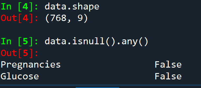
data.shape
data.isnull().any()
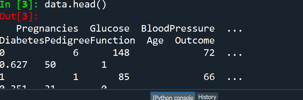
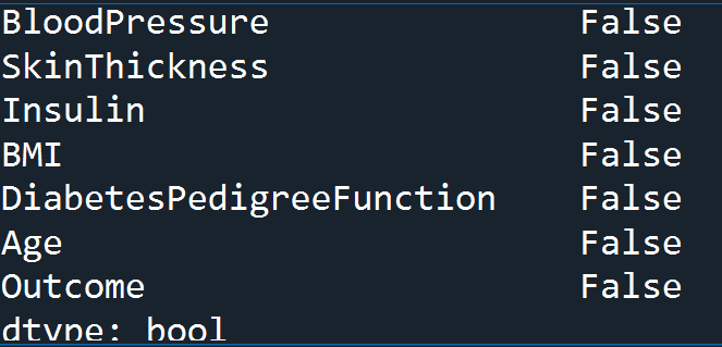
First of all, we have imported NumPy package which stands for numerical python which is the basic package for numerical calculation. Pandas library has been imported to work with dataframes. Matplotlib is a plotting library used to create 2D graphs and plots. Similarly, seaborn is also a plotting library used to provide a high-level interface for drawing informative statistical graphics. After importing the necessary libraries, we have loaded the diabetes dataset and read the dataset through dataframe data.
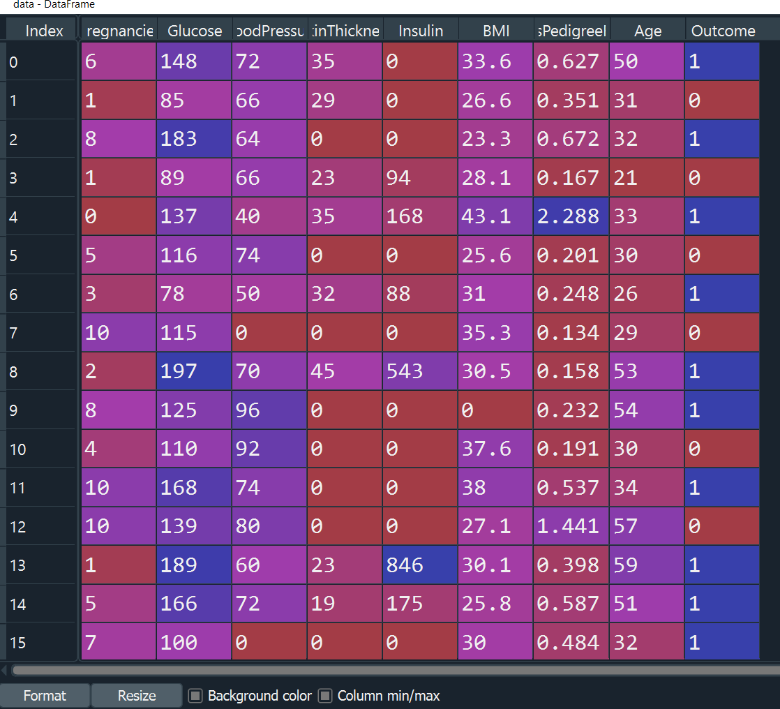
Spyder IDE has been used to write the codes. Dataframe ‘data‘ has been created with 768 rows and 9 columns. The head() function displays the top 5 rows, and isnull().any() function has been used to find if there is any null value, it returned false. The dataset contains 9 columns viz. pregnancies, glucose, blood pressure, skin thickness, insulin, BMI, diabetes pedigree function, age, and outcome. The outcome is the target variable, the rest all are the predictor variables.
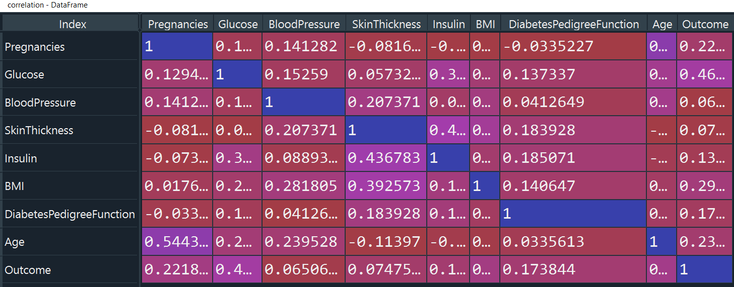
sns.pairplot(data,hue='Outcome')
plt.show()
correlation=data.corr()
correlation
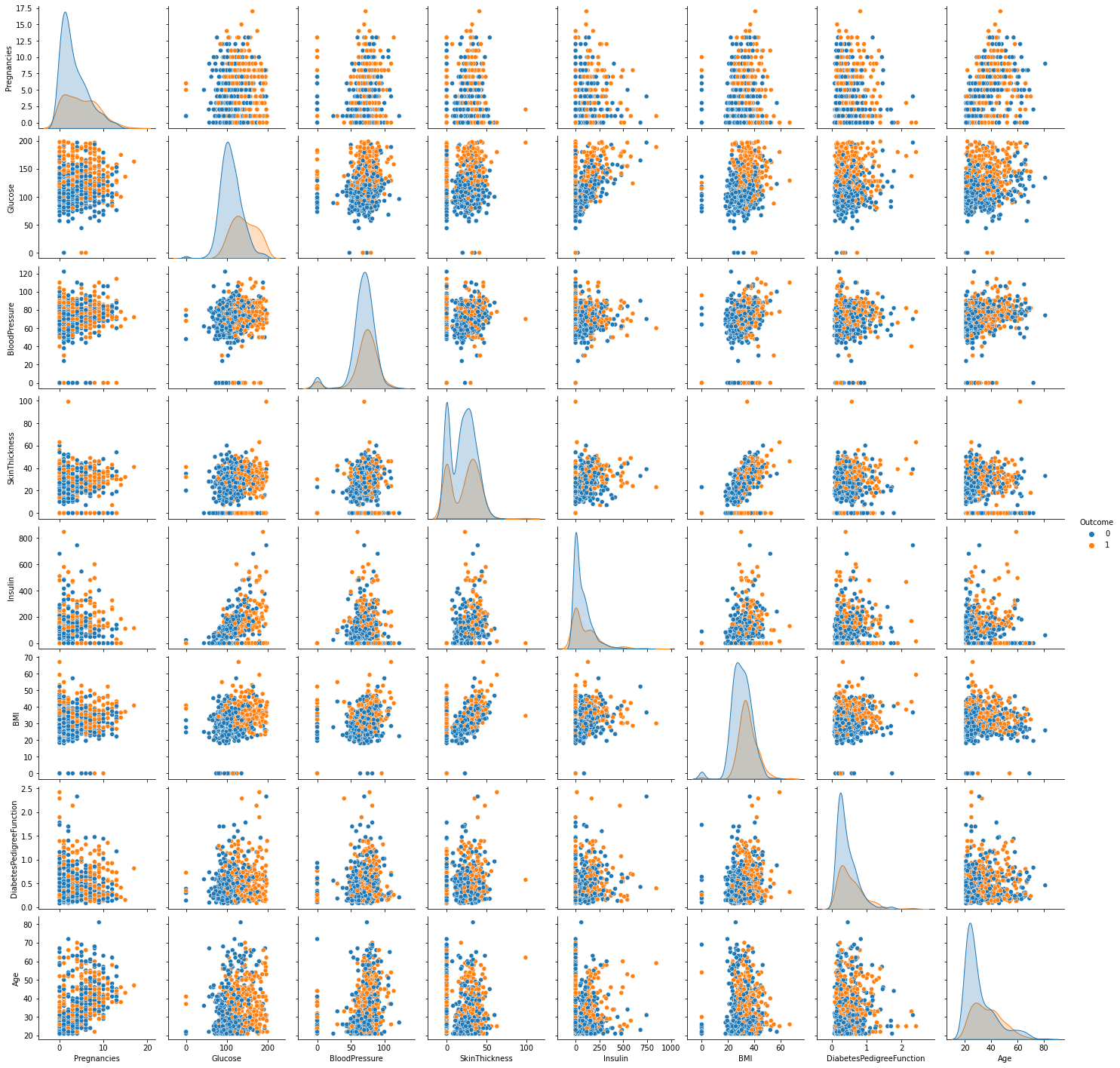
A pairwise plot has been used to create pairwise relationships in a dataset. It creates scatter plots for joint relationships and histograms for univariate distributions. The dataset comprised all female patients who are diabetic for 21 years and binary target variables, Outcome takes values 0 or 1 where 0 indicates negative for diabetes and 1 indicates positive for diabetes.
Correlation tells us about the strength of association between two variables. It lies between 0, no correlation, and 1, maximum correlation. It tells about how strong is the association between two variables.
y=data['Outcome']
x=data.drop(['Outcome'],axis=1)
from sklearn.model_selection import train_test_split
x_train,x_test,y_train,y_test=train_test_split(x,y,test_size=0.25,random_state=14)
x_train.shape,y_train.shape
x_test.shape,y_test.shape
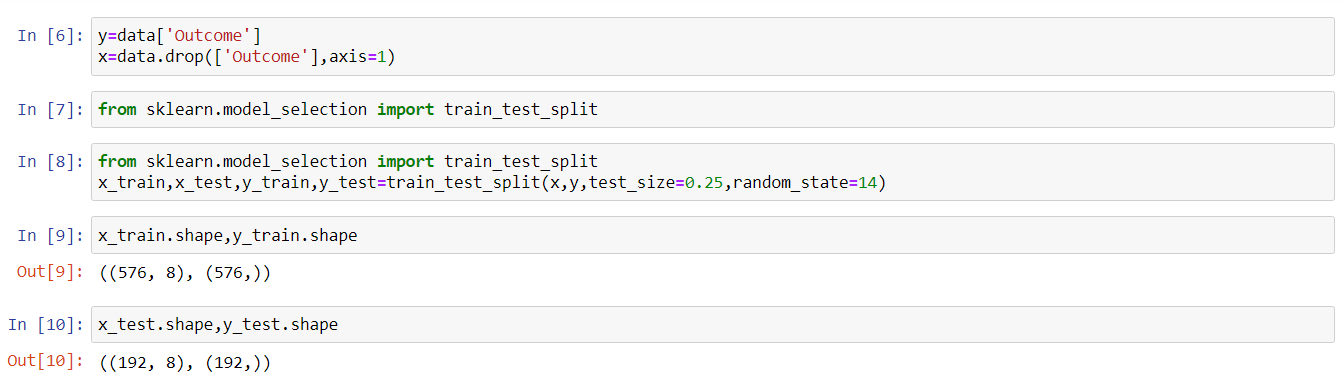
Now, the dataset was split into testing and training datasets by importing train_test_split module from Sci-kit learn library. The test size was 25% of the dataset, and the remaining part of the dataset was for training. Jupyter notebook was used for the core machine learning part henceforth.
from sklearn.tree import DecisionTreeClassifier
dt_model = DecisionTreeClassifier(random_state=14)
dt_model.fit(x_train,y_train)
dt_model.score(x_train,y_train)
dt_model.score(x_test,y_test)
from sklearn.metrics import confusion_matrix
tree_pred=dt_model.predict(x_test)
confusion_matrix(y_test, tree_pred)
tree_pred1 = dt_model.predict(x_train)
confusion_matrix(y_train, tree_pred1)
The dataset was tested through two classification tools which are Decision Tree and Logistic Regression. Both are imported from sci-kit learn library. The training set was fitted into the model, and scores for both training and testing sets were obtained. Then, the confusion matrix was imported from sci-kit learn. The confusion matrix is used to evaluate the accuracy of classification. The first column and first row represent True Positive, the second column and first row represent False Positive, the second row and first column represent False Negative, and the second row and second column represent True Negative.
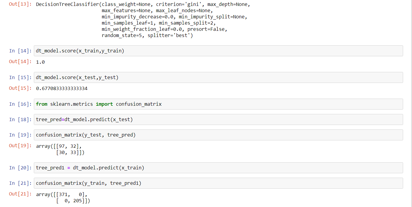
The score of the training model was a magnificent 100% which means it classified all the elements correctly as is evident as a result of the confusion matrix. But, a score of the testing model was 68% approximately. As can be seen with the help of the confusion matrix there was misclassification. This decision tree model was improved through the implementation of various measures.
from sklearn.linear_model import LogisticRegression
dt_model = LogisticRegression()
dt_model.fit(x_train,y_train)
dt_model.score(x_train,y_train)
dt_model.score(x_test,y_test)
reg_pred=dt_model.predict(x_test)
confusion_matrix(y_test, reg_pred)
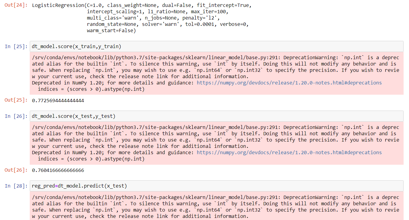
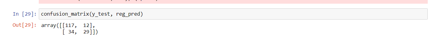
Logistic Regression was imported from sci-kit learn library. By adopting, similar procedures of Decision Tree, it can be seen that both the training and testing dataset were balanced. In the confusion matrix analysis for the testing dataset, it was observed that very few elements were misclassified compared to the Decision Tree model. So, the Logistic Regression model performed better.
Let us improve the Decision Tree model now
train_accuracy = []
test_accuracy = []
for depth in range(1,7):
dt_model=DecisionTreeClassifier(max_depth=depth, random_state=14)
dt_model.fit(x_train,y_train)
train_accuracy.append(dt_model.score(x_train,y_train))
test_accuracy.append(dt_model.score(x_test,y_test))
frame = pd.DataFrame({'max_depth':range(1,7),'train_acc':train_accuracy,'test_acc':test_accuracy})
frame
dt_model=DecisionTreeClassifier(max_depth=4,max_leaf_nodes=10,random_state=5)
dt_model.fit(x_train,y_train)
dt_model.score(x_train,y_train)
dt_model.score(x_test,y_test)
!pip install graphviz
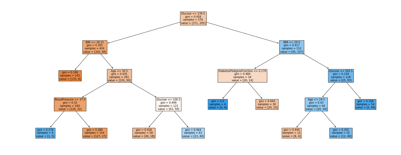
from sklearn import tree
plt.figure(figsize=(15,10))
tree.plot_tree(dt_model,filled=True,feature_names=x_train.columns)
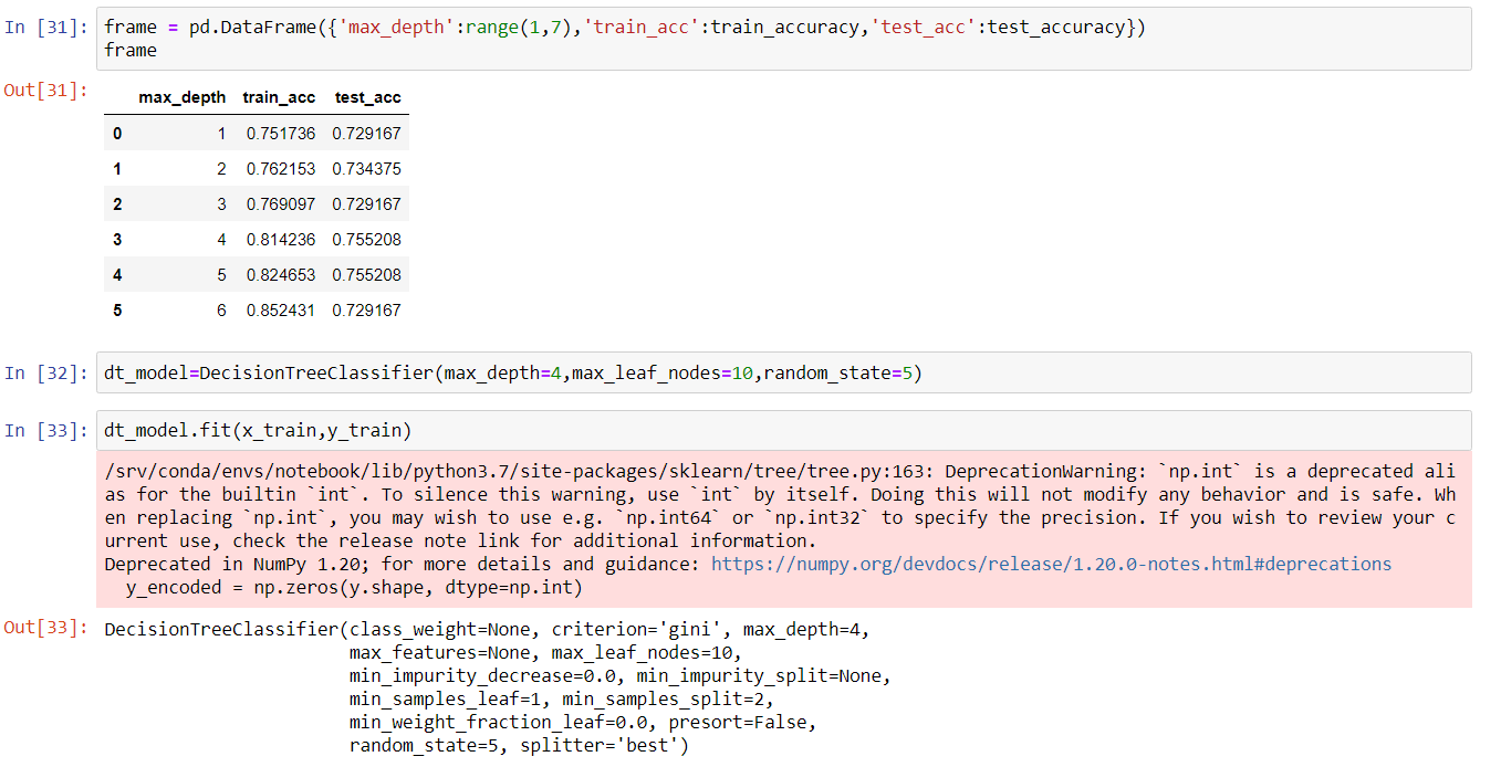
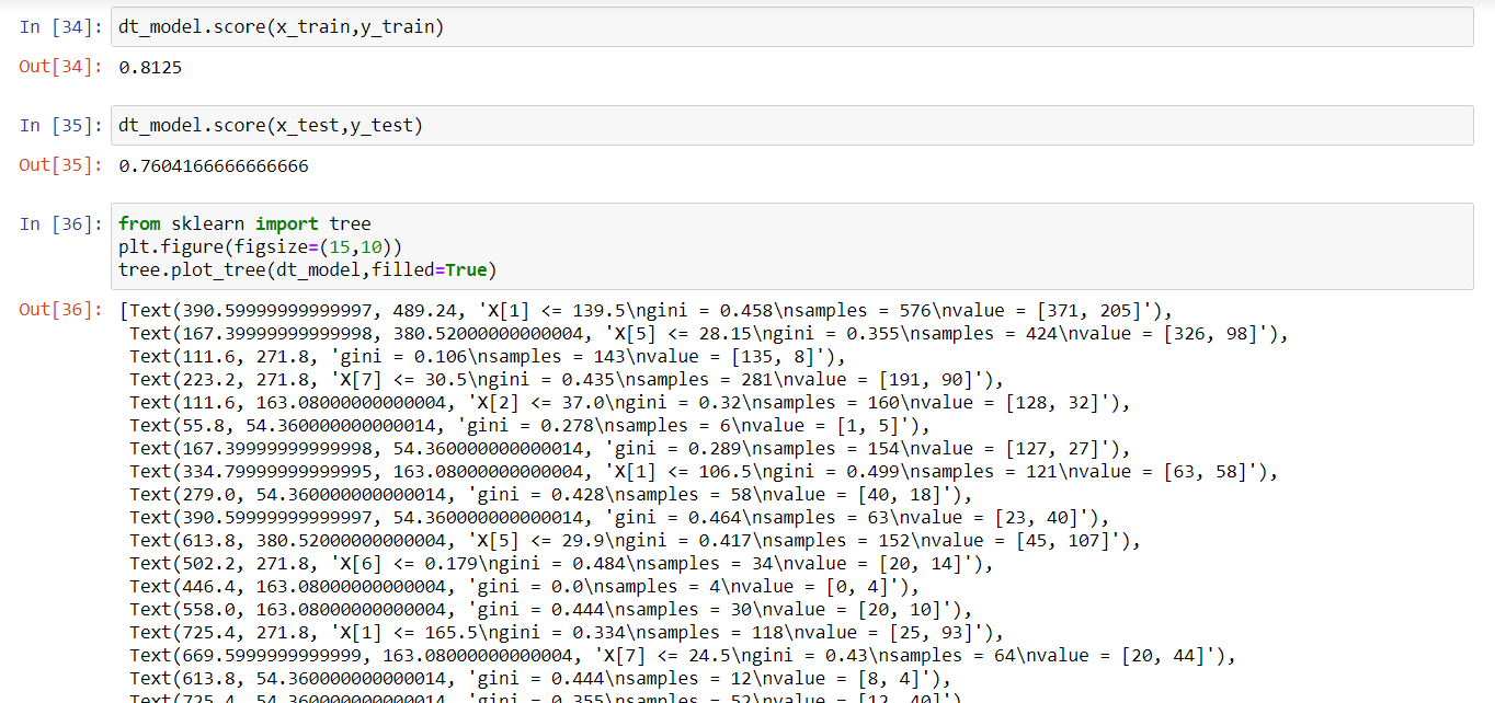
A decision Tree allows us to change certain parameters for the betterment of our model. In this model, we changed the maximum depth of the decision tree, fixed maximum leaf nodes, and changed the random state. It can be observed that the model performed better with an 81% score compared to that of 68%.
The tree was imported from sci-kit learn and the plot can be seen. The leaf nodes are split according to Gini Impurity which is a measure of the heterogeneity of the dataset. Gini Impurity of the pure dataset is 0.
Conclusion
Machine Learning models if synchronized properly with the knowledge of anatomy and physiology, clinical parameters, laboratory parameters, and medicines can prove to be a game-changer in the ongoing fight against diabetes.
Thank You for your valuable time
References
1. Pandey, S. K., & Sharma, V. (2018). World diabetes day 2018: Battling the Emerging Epidemic of Diabetic Retinopathy. Indian journal of ophthalmology, 66(11), 1652–1653. https://doi.org/10.4103/ijo.IJO_1681_18
2. https://www.kaggle.com/uciml/pima-indians-diabetes-database
The media shown in this article are not owned by Analytics Vidhya and are used at the Author’s discretion.


