Feature Transformation CheatSheet

Introduction

As is known, a proper feature transformation can bring a significant improvement to your model. Sometimes feature transformation is the only way to gain a better score, so it is a crucial point how you represent your data and feed it to a target model. In this article, I would like to go through some common data types and analyze various data transformations. For these purposes, I am going to use a GlobalLandTemperatures_GlobalLandTemperaturesByMajorCity.csv dataset which represents global climate changes from 1750 to 2015 years.

This dataset consists of very frequent feature types such as date, location, numerical and categorical columns. In this review, we will save for later a discussion about feature selection and various angles of feature engineering, as here we have a straight focus on possible ways of encoding such data. It is supposed to be a cheatsheet template that one might use when dealing with feature transformations in similar cases.

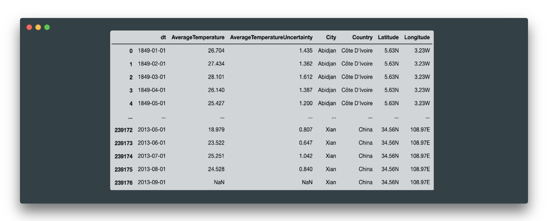
As a starting point, here is a quick look at the overall dataset statistics:

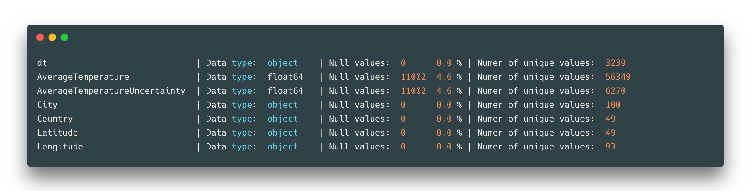
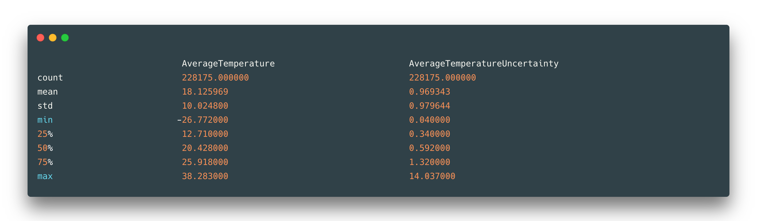
The dataset has no duplicated rows. Here are only two numerical features of type float64 and the rest are object types (some of them have to be converted to exact type). We can see that only these two numerical features AverageTemperature and AverageTemperatureUncertainty have 11002 null values each. And general statistics for these temperature values:

Imputation of missing values

First of all, let’s deal with missing values. It is a very common case where data has blank fields, random characters, and even wrong information. Here we suppose we have a more or less cleaned dataset with some null values. If you have some idea about your dataset and knowledge of where these missing values come from, then it would be easier for you to guess how to treat them.

On the other hand, in loads of cases, you are not sure and have to choose a method to fix your missing values. Why should we take attention to that? The simple answer is that not every machine learning algorithm can manage missing values. Another point of view is that with proper imputation/deletion you again can gain a better result. Here are few ideas to transform your missing values into something more informative:

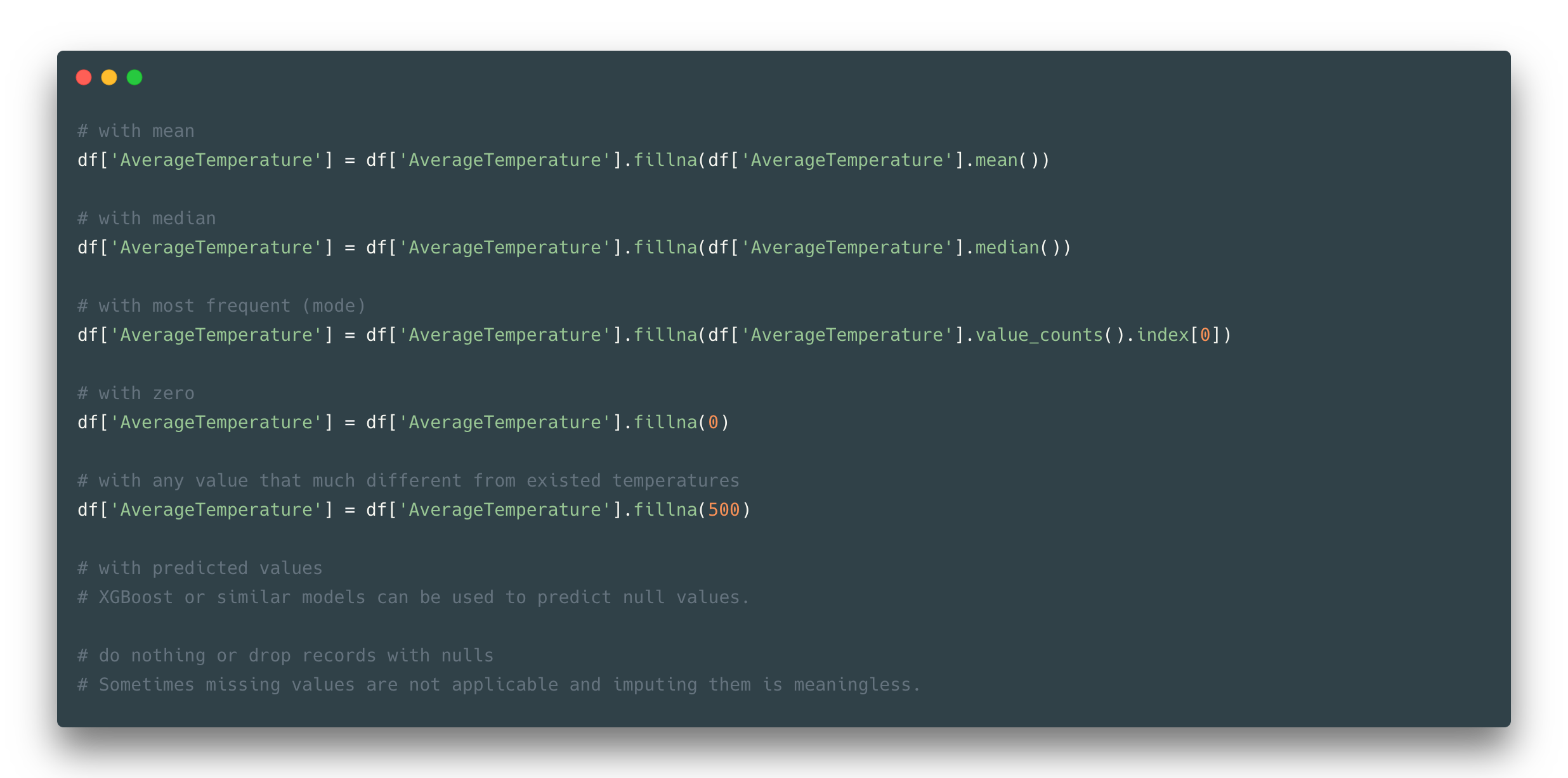
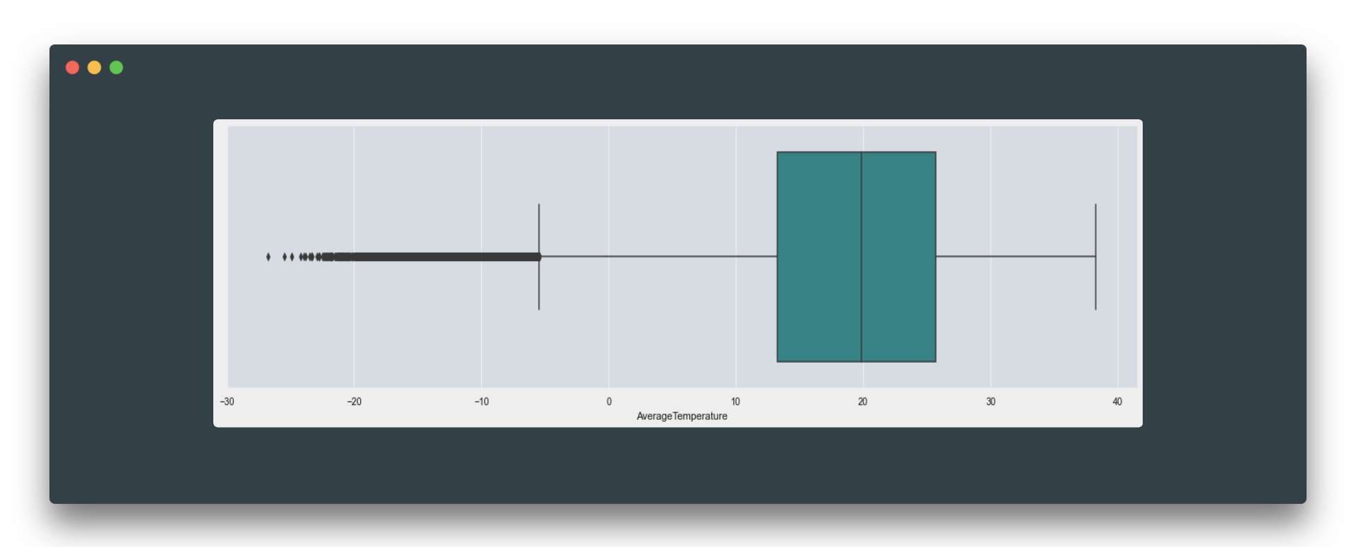
One way to go is to impute these missing values with median, mean, or mode (most frequent value). To choose between these three just take a look at a boxplot and distribution. If your data distributed symmetrically, then replacing missing data with mean might be a good idea. If your data is skewed or contains outliers, try to look into the mode or median imputation options.

There is also a common option to replace missing values with 0 or with any constant value way more different from existing in a given feature. It’s not always appropriate to fill nulls with 0 as there could be some zero values already (like in this example with temperature) and that would just mean a piece of wrong information.

If you have a large dataset and a little number of rows with nulls, it might be fine to remove these rows at all. Otherwise, there is also an option to predict missing values, and at this point, you should ask yourself if it is worth trying so (in the matter of time and efficiency). In our example let’s go for the median option.

Transforming numerical features

In the example dataset, AverageTemperature is a continuous feature because its value can assume any value from the set of real numbers. The option is to make it be more discrete – to create classes for several temperature ranges.

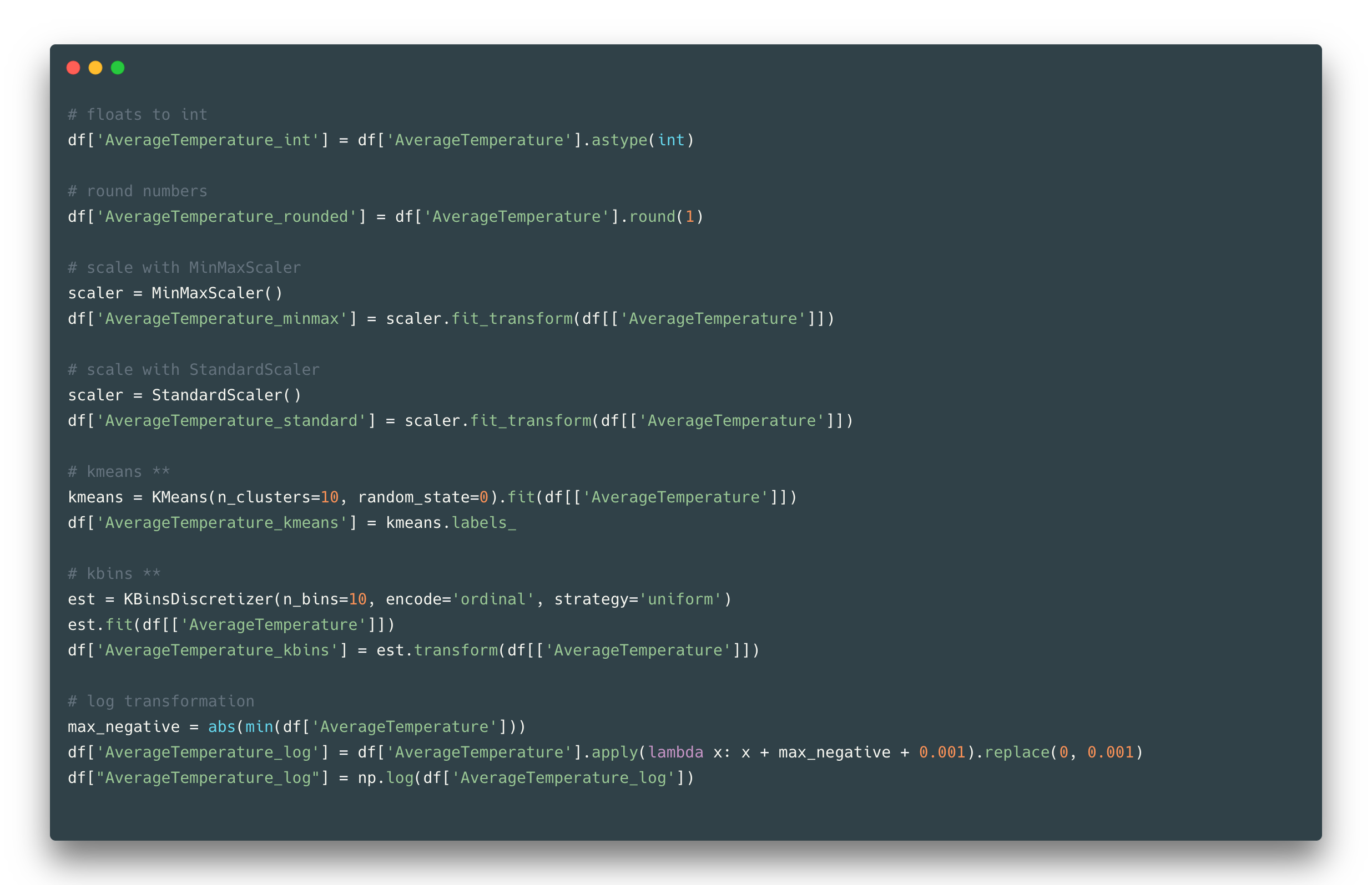
The easy way is to convert your floats to ints, or round it by some decimal. Another way to make classes out of feature values is to apply quantization methods like K-means. One is dividing values into k clusters in which each value belongs to the cluster with the nearest mean, and another just binning continuous data into k intervals.

These methods help to change the distribution of initial values which might be useful for example to fix outliers problems. The k number of clusters/bins sometimes can be complicated to choose from, in such cases, one might use the Silhouette coefficient or Elbow method to find an optimal k value. Another way of numerical feature transformation is scaling. When your features are in different scales it is a good practice to transform them all into one scale.

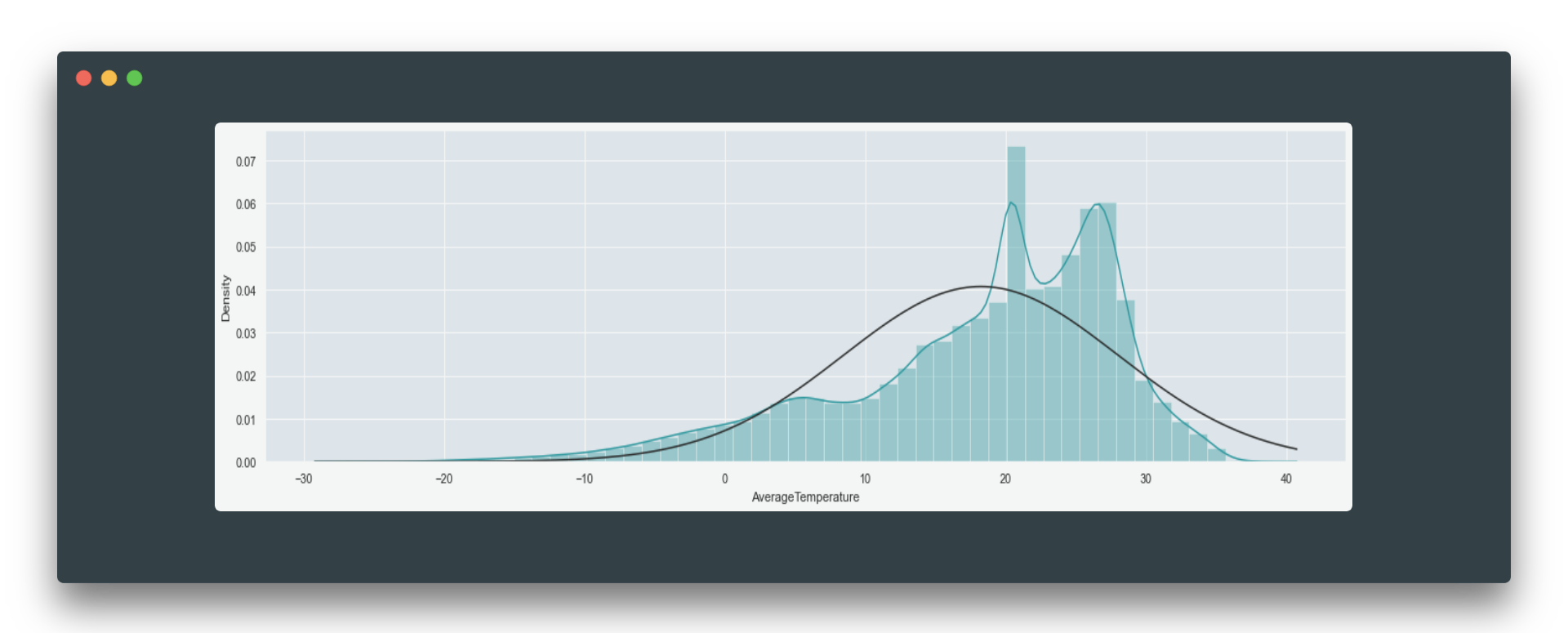
In such case units of the model, coefficients are going to be the same, therefore they all bring equal contribution into the analysis. Scaling could also fasten the convergence and show a better performance. One more popular technique to change your feature in a meaningful way is a log transformation. It is used to transform skewed data to make it looks more like a normal distribution.

Before log transformation:

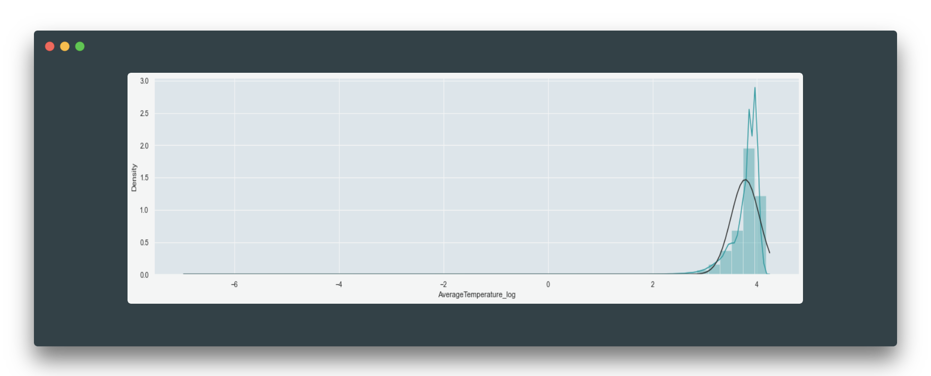
And after:

If you noticed the scaling results are not satisfactory, check the distributions of the data again to come up with a better method for feature scaling. Once you did a means or similar technique to reduce the number of unique values in a feature, you might want to proceed with further encoding e.g., create dummies:

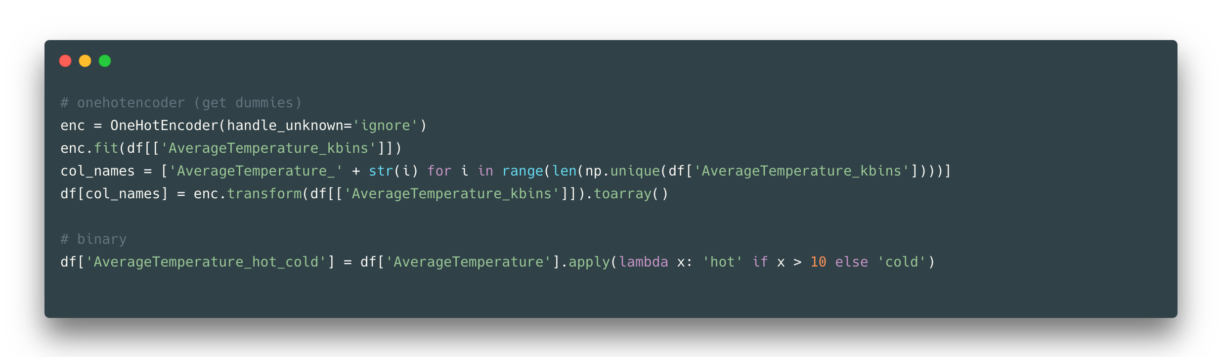
One hot encoding helps to make your classes be equal for the model by creating a binary feature per each (so that a model would not be able to assign more importance to class number 100 than to class number 1). Or just simply binarize your feature or make two labels only, although it reduces a lot of information, in some cases, it might be helpful.

Datetime feature transformations

Datetime is a common type of feature that can be transformed in different ways, so let’s first look at its ‘date’ part.

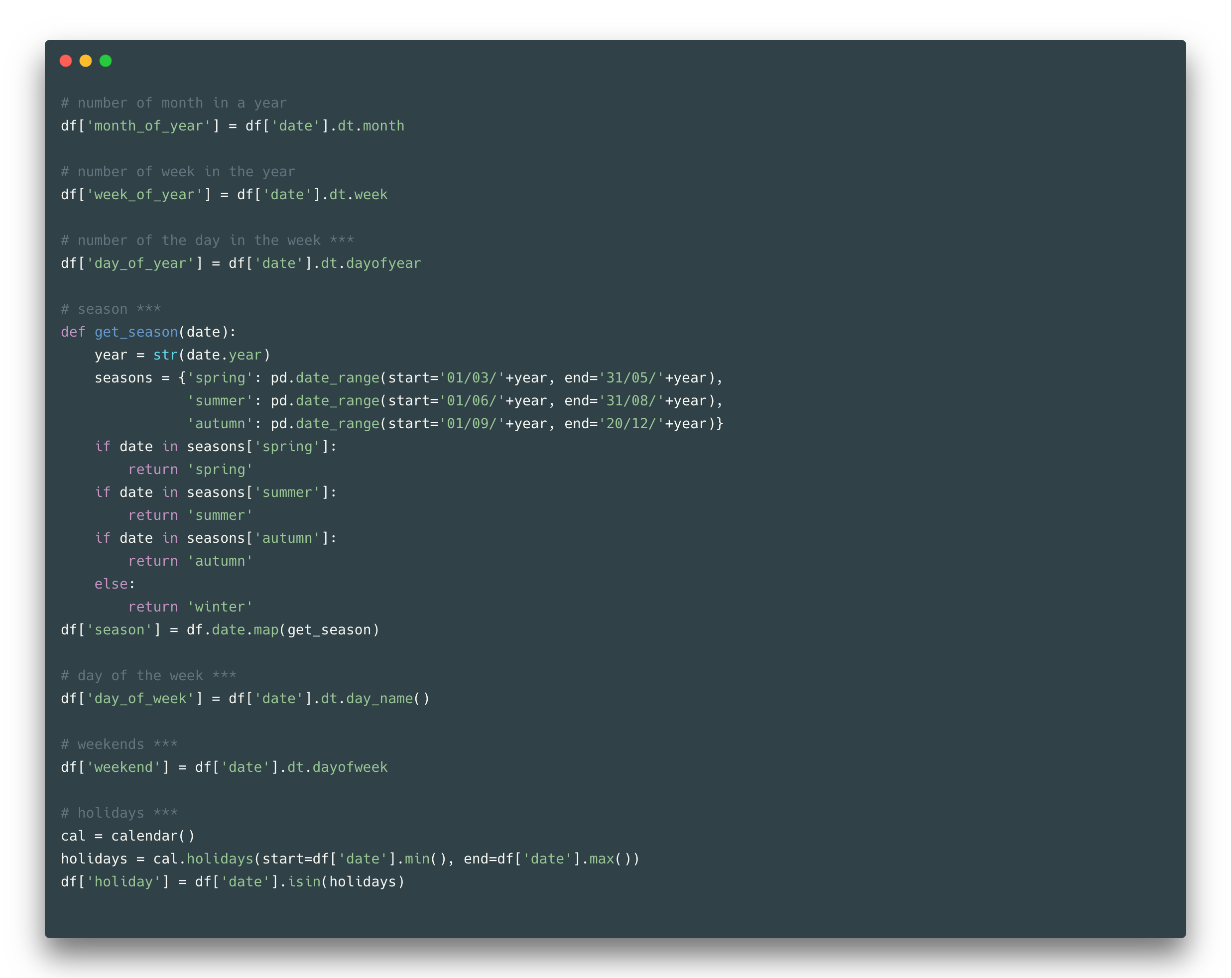
Date

The most efficient way to transform data into something meaningful might be to divide it into the year, season, month, week, and day. Furthermore, a day could be defined as a day of the year, day of the week, or month. It can be a weekend day, holiday, or just the usual working day. Here you should be aware that in each country/hemisphere these weekends/holidays/seasons may vary and it might not be a good idea to apply one rule to all the countries.

 

Time

Time can also be separated into hours/minutes/seconds/etc and to which units to convert depends on the specifics of your dataset. Hours can also be defined as a part of a day, meaning that it can be a binary feature with two Day/Night values or it can consist of more labels as in the example:

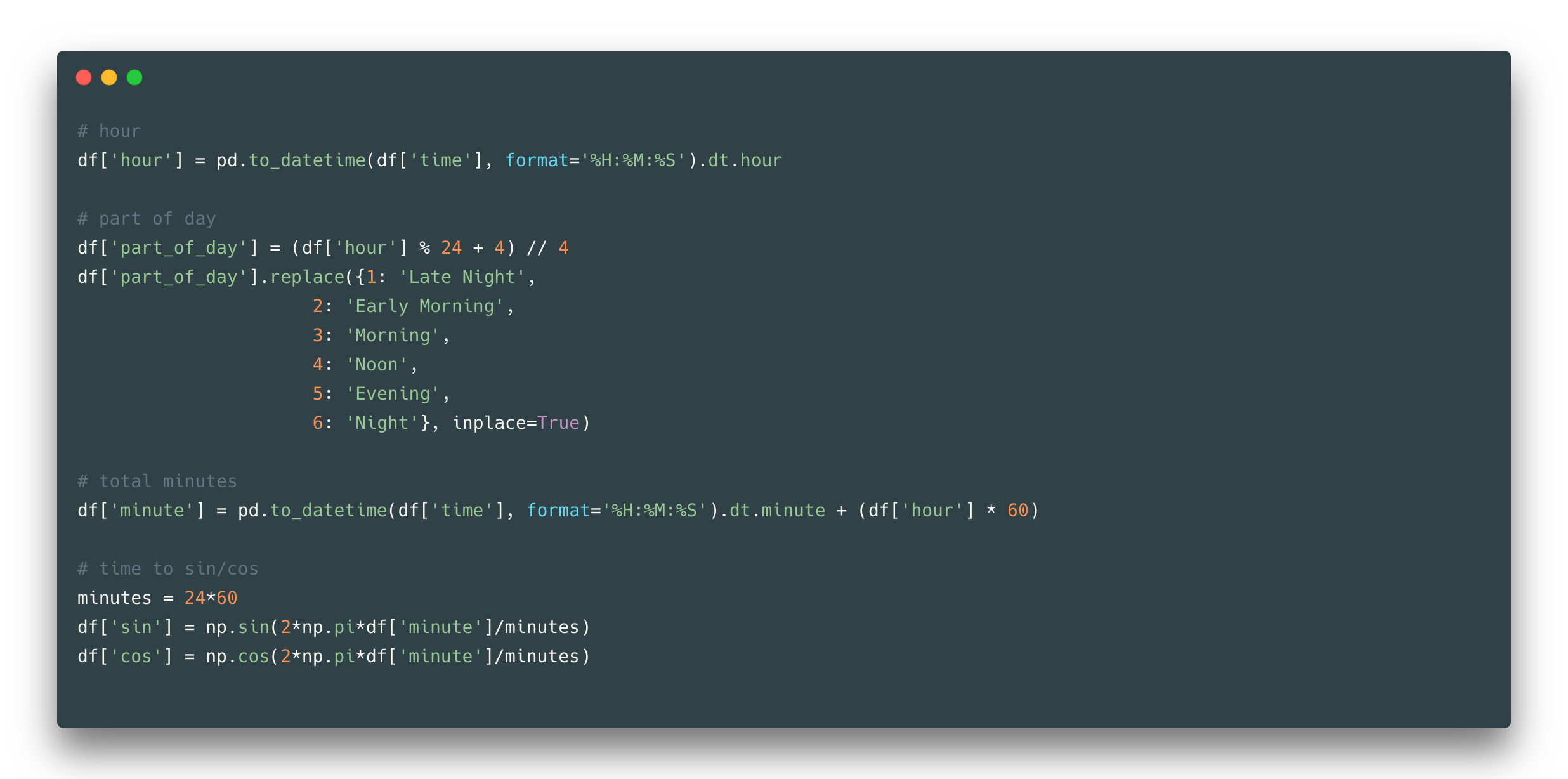
Another stunning time transformation (that can be applied to any circular features) is to convert time to sin and cos. Though it creates two features in exchange for one, it still can be useful when taking into account the difference in time between the end of one day and the start of another day (with sin-cos features there will not be a gap as it is between 23 hour and 00 hour next day).

Geographical feature transformation

Geolocation can be presented in many different ways, but here let’s show the most common option with latitude and longitude, given that in the dataset it is presented in latitude N/S and longitude E/W form (e.g. 5.63N, 3.23W).

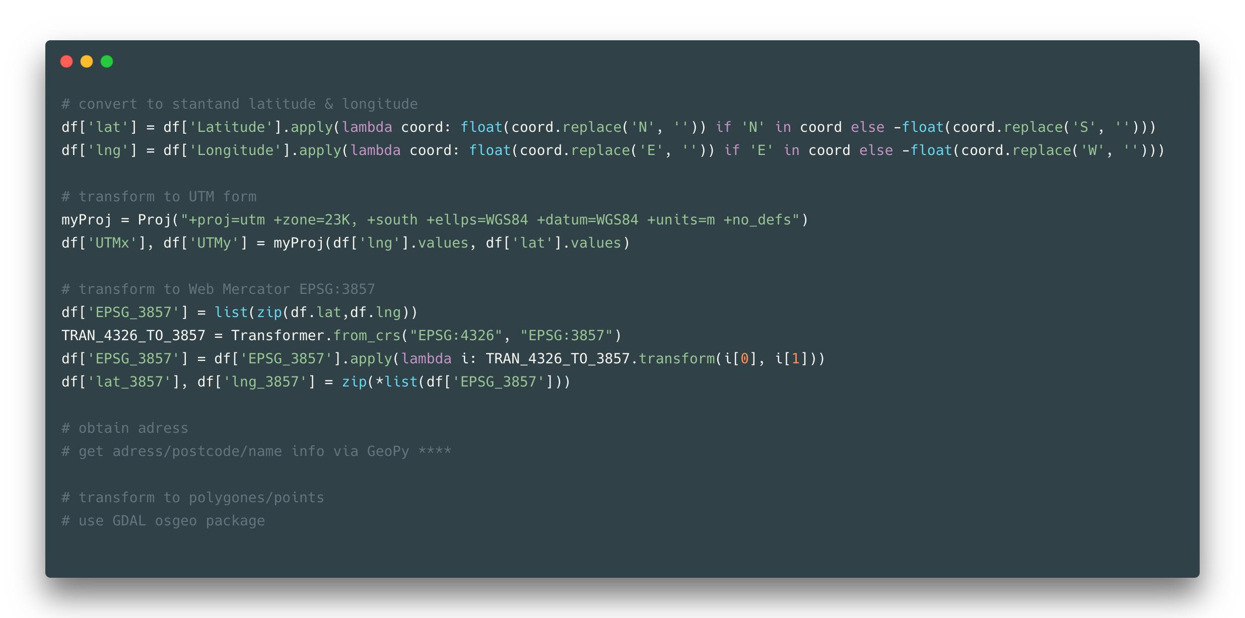
First, you might want to convert these coordinates to standard form (meaning that they become numerical, which is good). And afterward, there is a huge range of different projections and coordinates variations you might be interested in. You might consider one of those is the most suitable in your case, but in the most general way, you would only use the web Mercator form.

Another useful transformation is to obtain an address from your coordinates, which might include country name, city, street, house, name of the place, postcode, and other things. Sometimes you might need to create a zone of locations and therefore you transform your coordinates to polygons and points of polygons.

Text transformation

One of the most common feature representations is a text. It could be plain text, just some phrases, words, or any structured and unstructured number of characters. For example, in the observed dataset, there is a Country column consists of country names. What could be done about it? Not much in our case as this column is more about labels than the text itself, but still, you might notice the names in the Country column are not all in the English language (e.g. Côte D’Ivoire country name), and, for example, you might want to have all your records in one language.

 

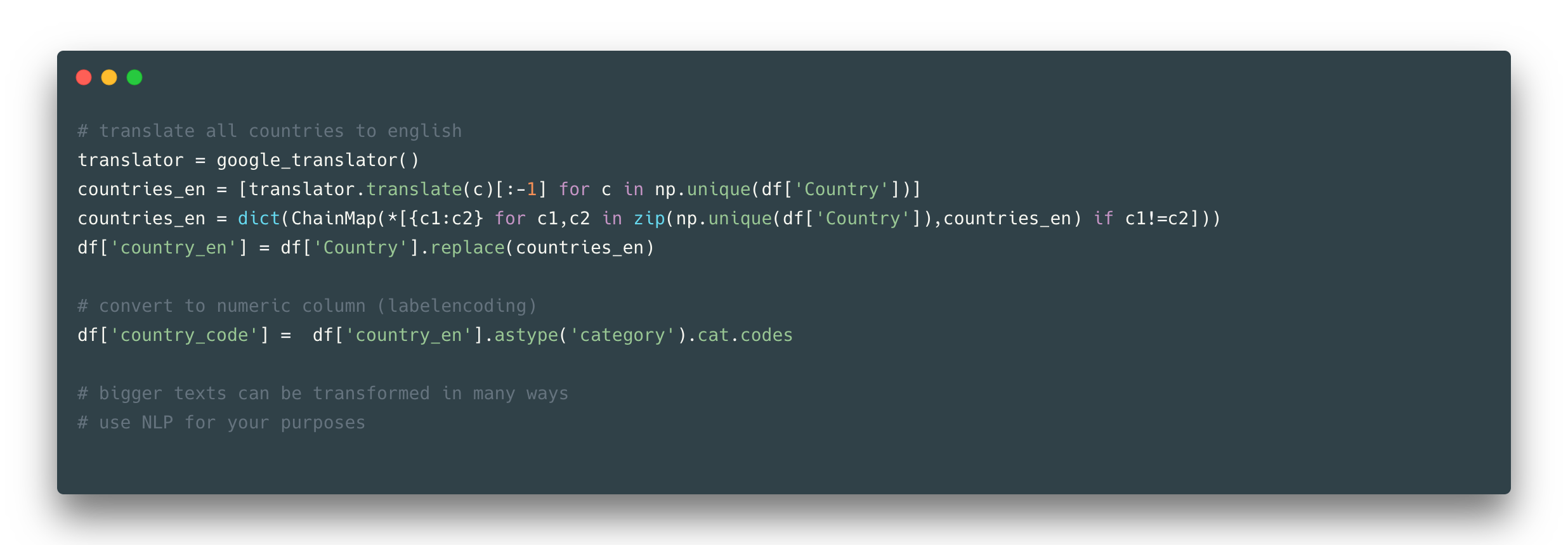
So that would be a good transformation – to translate all country words to one language. For more complicated cases you might want to use regex and NLP methods to deal with textual data.

We went through the most common feature types you might face in your day-to-day routine and suggested a good practice to manage transformation for such features. This cheatsheet is a reminder that there are plenty of ways of converting features to some efficient useful information and it is better not to stick to one and only transformation with different models, but to look at the transformation from different sides.

Thanks for reading! Please leave a comment if you have any feedback.

Full code for this article can be found here

Asya Evloeva 06 Apr 2021