Introduction to Audio Classification
This article was published as a part of the Data Science Blogathon
Introduction
Audio classification or sound classification can be referred to as the process of analyzing audio recordings. This amazing technique has multiple applications in the field of AI and data science such as chatbots, automated voice translators, virtual assistants, music genre identification, and text to speech applications.
Audio classifications can be of multiple types and forms such as — Acoustic Data Classification or acoustic event detection, Music classification, Natural Language Classification, and Environmental Sound Classification.
In this article, we will explore audio classification through a detailed hands-on project.

We will be implementing Audio classification by using the TensorFlow machine learning framework. We would be taking into account a raw audio dataset and categorized it into speech and music. Followed by pre-processing, creating, and training a deep learning model to perform classification. This way we can classify incoming audio in one of the two classes, in either speech or music.
Nowadays even though we are surrounded by all kinds of sounds, This domain remains overshadowed by image classification. One of the reasons for that could be the type of pre-processing required for audio is not as straightforward as image data.
Usually, we convert the audio signal from raw audio into two spectrograms before being fed into the models. And this is what we would learn upon successfully implementing the project!!
Learning Objectives
- Environment setup
- Data exploration
- Creating spectrogram
- Data pre-processing
- Model creation
- Model Training
- Predictions
Setting up the environment
Installation
Install the package via pip which is used by TensorFlow datasets to download
and extract the specific data set that will be used.
!pip install -q pydub
Imports
Import the required libraries that would be used throughout the project.
import tensorflow as tf
import tensorflow_datasets as tfds
from tensorflow.keras.layers import Input, Lambda, Conv2D, BatchNormalization
from tensorflow.keras.layers import Activation, MaxPool2D, Flatten, Dropout, Dense
from IPython.display import Audio
from matplotlib import pyplot as plt
from tqdm import tqdm
Data Loading
We would use TensorFlow datasets to load a specific dataset known as gtzan_music_speech, which is a Music speech data set. It will take a few seconds to download and extract the data set.
dataset = tfds.load("gtzan_music_speech")
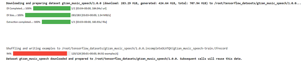
This data set consists of 128 audio files. Each is 30 seconds long and music and speech classes are having 64 audio files each. Here, each second of audio playback means 44,100 samples are being played.
Data Exploration
After the data is downloaded we can move ahead and explore the data. Notice that there is no separate split for validation or a test set in this dataset. It comes with just the training set consisting of 128 files.
Let us create a training data set and an iterator.
train = dataset["train"]
idata = iter(train)
We can iterate forward and see that the first key is audio. We can listen to this live audio using the following lines of code. We can set the sample rate in the audio class, here we set it as 22,050.
ex = next(idata)
audio = ex.get("audio")
label = ex.get("label")
Audio(audio, rate= 22050)
This audio bar will be the output after executing the commands and can be used to play the audio.
Moving forward we can set labels as 0 and 1. Zero corresponds to music class and one corresponds to speech. Create dictionaries to convert indices to classes and classes to indices.
index_class = {0: "music", 1: "speech"}
class_index = {"music" : 0, "speech": 1}
Create a function to plot the audio file.
def plot_wave(audio):
    plt.plot(audio)
    plt.xlabel("samples")
    plt.ylabel("amplitude")
    plt.show()
plot_wave(audio)
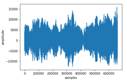
The X-axis shows there are over 650,000 samples. From this, we can conclude that we won’t be able to use this audio in its raw form.
So we would be transforming this audio data in another way in a feature that is more conveniently consumed in a neural network such as a spectrogram.
Creating Spectrogram
A spectrogram is a visual way of representing the signal strength of a signal over time at various frequencies present in a particular waveform.
In our case, we can consider the raw audio signal as a vector with 650,000 or so dimensions. To make the input more manageable, we split the audio into smaller chunks.
Create a function that will provide a short time to transform the audio signal. We can specify the frame length as “256”, frame step as “512” which is the number of samples between two consecutive frames starting points.
So if the first frame starts from zero and ends at the sample
number 2048 then the next frame will start at 512.
def stft(audio, frame_length = 2048, frame_step=512, fft_length=256):
    return tf.signal.stft(
    tf.cast(audio, tf.float32),
    frame_length= frame_length,
    frame_step= frame_step,
    fft_length= fft_length
    )
audio_stft = stft(audio)
audio_spec = tf.abs(audio_stft)
Now we’re going to consider the magnitude of the stfd and ignore the face content.
Create a function that will plot the spectrogram. And let us view the first 200 values.
def spec(spec):
plt.figure(figsize=(12,14))
plt.imshow(tf.transpose(spec), cmap= "viridis")
plt.colorbar()
plt.show()
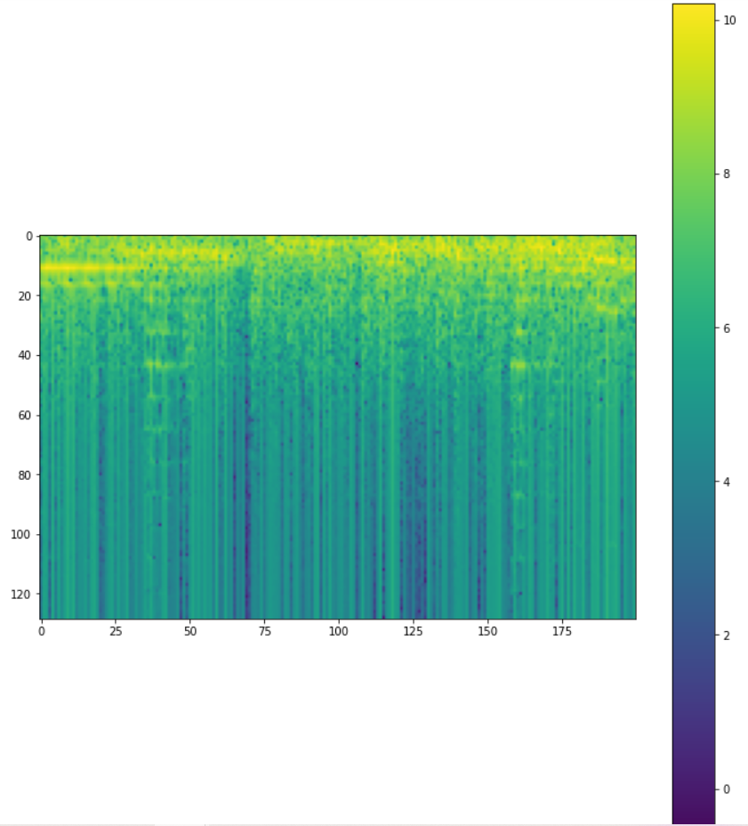
spec(audio_spec[:200])
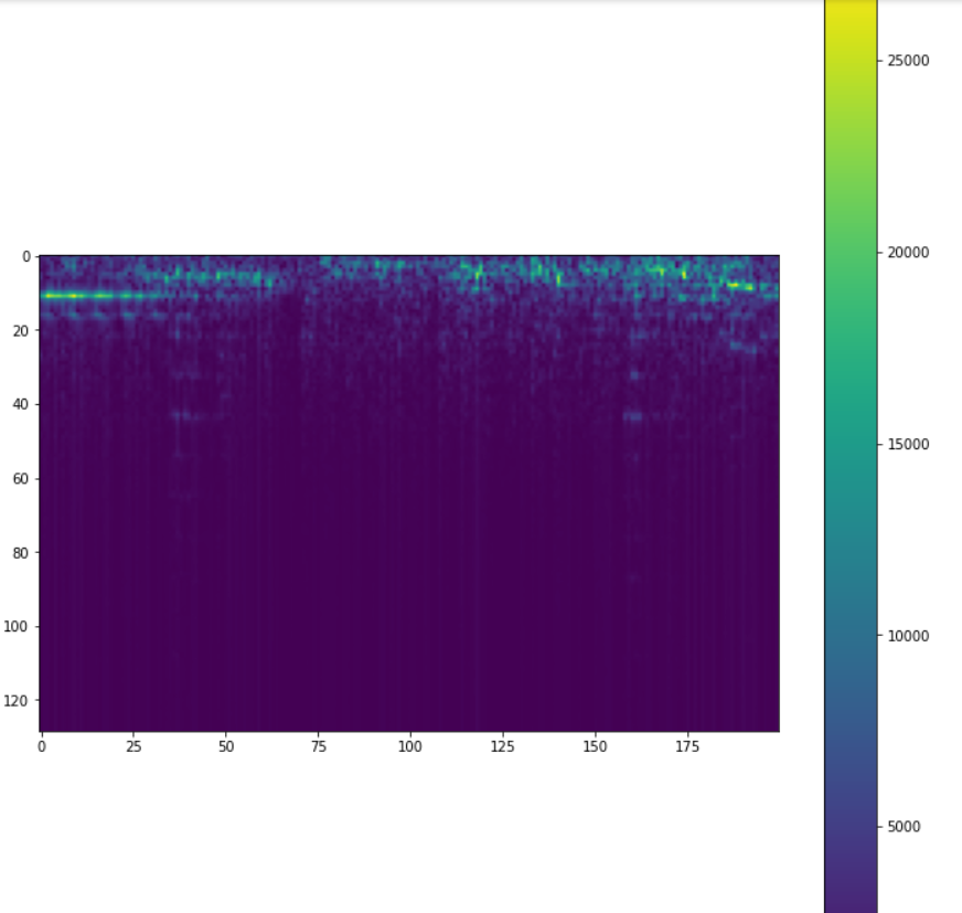
Here we can see that there’s a lot of energy concentration in the first few frequency bins and a colour bar is displayed reflecting the amplitude values in different frequency bins.
Let us plot a log spectrogram, this shows that the colour bar now values to a much better range. This corresponds to how human hearing works.
audio_spec_log = tf.math.log(audio_spec)
spec(audio_spec_log[:200])
And finally, we create a spectrogram function, which is nothing more than what we have already done, but it just wrapped inside a function. We pass in audio then stft is calculated, the absolute value is taken to get the spectrogram
and then we compute a log after transposing that spectrogram.
def spectrogram(audio):
    audio_stft = stft(audio)
    audio_spec = tf.abs(audio_stft)
    return tf.math.log(tf.transpose(audio_spec))
Finally, we have converted raw audio into an image-like representation, which encodes the frequency and amplitude information overtime of the raw audio signal. Here, the color represents the amplitude as the color bar indicates different frequency bands over a period of time.
The main idea is that if we consider 5-second audio, then we will be able to predict if that chunk is speech or music if it’s too short then we might not be able to do that, but five seconds is good enough.
And this way, instead of using one audio file as a single example, we get more examples out of that.
Data Preprocessing
Create a function that will take one example and form a batch of examples out of that single example. This will break the audio into 6 chunks.
sr =22050
chunk = 5
def preprocess(ex):
    audio = ex.get("audio")
    label = ex.get("label")
    x_batch, y_batch = None,None
    for i in range (0, 6):
        start = i * chunk * sr
        end = (i + 1) * chunk * sr
        audio_chunk = audio[start: end]
        audio_spec = spectrogram(audio_chunk)
        audio_spec = tf.expand_dims(audio_spec, axis=0)
        current_label = tf.expand_dims(label, axis=0)
        x_batch = audio_spec if x_batch is None else tf.concat([x_batch, audio_spec], axis=0)
        y_batch = current_label if y_batch is None else tf.concat([y_batch, current_label], axis=0)
        return x_batch, y_batch
Now we are going to iterate over it and get the batches for each example and are going to vertically stack them with X train.
x_train, y_train = None, None
for ex in tqdm(iter(train)):
    x_batch, y_batch = preprocess(ex)
    x_train = x_batch if x_train is None else tf.concat([x_train, x_batch], axis=0)
    y_train= y_batch if y_train is None else tf.concat([y_train, y_batch], axis=0)
The output shows that we have iterated over 128 files. Next, we create random indices and gather the x_train and y_train with the same indices. Then create a validation set and update the training set to exclude the validation set.
indices = tf.random.shuffle(list(range(0, 768)))
x_train = tf.gather(x_train, indices)
y_train = tf.gather(y_train, indices)
n_val = 300
x_valid=x_train[:n_val, ...]
x_valid=x_train[:n_val, ...]
x_train = x_train[:n_val, ...]y_train = y_train[:n_val, ...]
Finally, we can create multiple spectrograms and display some of them together. Certain differences can be identified in music spectrograms and speech spectrograms.
plt.figure(figsize=(12,12))
st=0
for i in range(0,6):
    x,y = x_train[st +i], y_train[st+i]
    plt.subplot(3,2,i+1)
    plt.imshow(x, cmap="viridis")
    plt.title(index_class[y.numpy()])
    plt.colorbar()
plt.show()
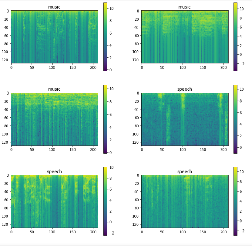
Visually we can observe really stark vertical lines in the speech spectrograms which are not that prominent in the music spectrograms.
Model creation
Let us start creating the model by considering the spectrogram features as image features. So we can create a simple convolutional neural network. We would be taking the spectrogram as input and perform some convolutions that help to recognize the features that are present in the spectrograms and based on that eventually predict the corresponding class.
input_ = Input(shape=(129, 212))
x = Lambda(lambda x: tf.expand_dims(x, axis=-1))(input_)
for i in range(0, 4):
    num_filters = 2**(5 + i)
    x = Conv2D(num_filters, 3)(x)
    x = BatchNormalization()(x)
    x = Activation("tanh")(x)
    x = MaxPool2D(2)(x)
x = Flatten()(x)
x = Dropout(0.4)(x)
x = Dense(128, activation="relu")(x)
x = Dropout(0.4)(x)
x = Dense(1, activation="sigmoid")(x)
model = tf.keras.models.Model(input_,x)
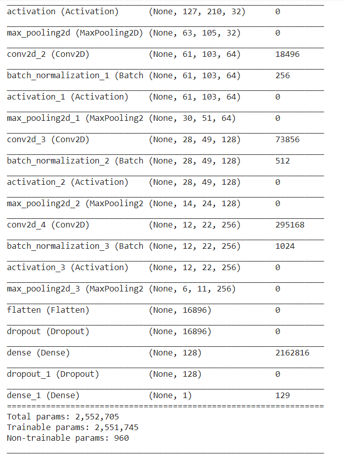
Create the first layer as an input layer followed by a convolution layer with a number of filters then we apply batch normalization, activation function, and Max pooling layer which reduces the dimension of the output.
Now we can flatten the output, drop out, and final 1 or 2 fully connected layers to get the output. This will be our final output layer, which has just one neuron and 6 as activation function because our labels are 0 or 1.
Let us compile the model and summarise it.
model.compile(
loss="binary_crossentropy",
optimizer= tf.keras.optimizers.Adam(learning_rate=3e-6),
metrics=["accuracy"]
)
model.summary()
Model Training
Create a function and set the desired accuracy, beyond that we don’t want to train the model so we cease the training as soon as the model achieves
the target accuracy for the validation set.
In case the validation accuracy at end of the epoch is higher than the accuracy target we will stop training.
class CustomCallback(tf.keras.callbacks.Callback):
def __init__(self, *args, **kwargs):
    super(CustomCallback, self).__init__(*args, **kwargs)
    self.target_acc = kwargs.get("target_acc") or 0.95
    self.log_epoch = kwargs.get("log_epoch") or 5
def epoch_end(self, epoch, logs=None):
    loss = logs.get("loss")
    acc = logs.get("accuracy")
    val_loss = logs.get("val_loss")
    val_acc = logs.get("val_accuracy")
    if (epoch + 1) % self.log_epoch ==0:
        print(f"Epoch: {epoch:3d}, Loss: {loss: .4f}, Acc: {acc:.4f}, Val Loss: {val_loss: .4f},Val Acc: {val_acc: .4f}")
    if val_acc >= self.target_acc:
        print("Target val accuracy", val_acc)
        model.stop_training = True
Now we fit the model by using a 12 batch size and set the number of epochs to 500.
_ = model.fit(
    x_train, y_train,
    validation_data= (x_valid, y_valid),
    batch_size=12,
    epochs=500,
    verbose=False,
    callbacks=[CustomCallback()]
    )
Note: It is advisable to use GPU for speeding the training process
Prediction
After training, we can perform predictions and get the classes by checking the predicted values. If they are greater than .5, the predicted class is one.
If they are less than .5, the predicted class is zero.
ex = next(idata)
x_test, y_test= preprocess(ex)
preds= model.predict(x_test)
pred_classes= tf.squeeze(tf.cast(preds > 0.5, tf.int8))
y_test
End Notes
Through this article, we have understood the basics of audio processing with TensorFlow for neural networks and there are a number of different features incorporated when it comes to audio and deep learning. We have determined the importance of spectrograms through practical implementation when it comes to Audio classification. This project can be extended to solve real-life complex problems.
The media shown in this article are not owned by Analytics Vidhya and are used at the Author’s discretion.


I am unable to download the dataset. it is giving me time out error.. Can you pls help?