Beta Distribution: What, When & How

By Krishna Kumar Tiwari, Data Science Architect at InMobi

Welcome to the series of W2HDS (What, When & How in Data Science). W2HDS comes with stories on topics which are in day to day use of a Data Scientists. Ideally is pretty simple and clear, a story will cover what, when and how of a data science concept. W2HDS series will cover multiple stories inside to cover the full concept end to end by following W2H concept. We will also have hosted notebooks where you can try these concepts by running each cells and try your experiments.

In this story, we will cover Beta Distribution.

 

What ?

 

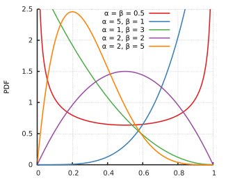
Beta distribution is a distribution of probabilities

Let's revise the probability, probability of an event can be calculated using below formula.

Many times in real life, we come up with scenarios when we don't know the actual probability but we have prior knowledge to guess the probability (called as prior in Data Science world), beta distribution can be used to represent all the possible values that probability can take.

Thanks to wikipedia for the definition.

In probability theory and statistics, the beta distribution is a family of continuous probability distributions defined on the interval [0, 1] parametrized by two positive shape parameters, denoted by α± and α², that appear as exponents of the random variable and control the shape of the distribution

 

I really like to thank David Robinson for explaining the beta distribution from a baseball angle. Here is simplest example to understand beta distribution, mostly everything here from David Robinson blog, as that is perfectly written.

Anyone who follows baseball is familiar with batting averages- simply the number of times a player gets a base hit divided by the number of times he goes up at bat (so it's just a percentage between 0 and 1).

.266 is in general considered an average batting average, while .300 is considered an excellent one.

Imagine we have a baseball player, and we want to predict what his season-long batting average will be. You might say we can just use his batting average so far- but this will be a very poor measure at the start of a season! If a player goes up to bat once and gets a single, his batting average is briefly 1.000, while if he strikes out, his batting average is 0.000. It doesn't get much better if you go up to bat five or six times- you could get a lucky streak and get an average of 1.000, or an unlucky streak and get an average of 0, neither of which are a remotely good predictor of how you will bat that season.

Why is your batting average in the first few hits not a good predictor of your eventual batting average? When a player's first at-bat is a strikeout, why does no one predict that he'll never get a hit all season? Because we're going in with prior expectations. We know that in history, most batting averages over a season have hovered between something like .215 and .360, with some extremely rare exceptions on either side. We know that if a player gets a few strikeouts in a row at the start, that might indicate he'll end up a bit worse than average, but we know he probably won't deviate from that range.

Given our batting average problem, which can be represented with a binomial distribution (a series of successes and failures), the best way to represent these prior expectations (what we in statistics just call a prior) is with the Beta distribution- it's saying, before we've seen the player take his first swing, what we roughly expect his batting average to be. The domain of the Beta distribution is (0, 1), just like a probability, so we already know we're on the right track- but the appropriateness of the Beta for this task goes far beyond that.

We expect that the player's season-long batting average will be most likely around .27, but that it could reasonably range from .21 to .35. This can be represented with a Beta distribution with parameters α±=81 and α²=219

I came up with these parameters for two reasons:

• The mean is α±/(α±+α²)=81+219=.270
• As you can see in the plot, this distribution lies almost entirely within (.2, .35)- the reasonable range for a batting average.

You asked what the x axis represents in a beta distribution density plot- here it represents his batting average. Thus notice that in this case, not only is the y-axis a probability (or more precisely a probability density), but the x-axis is as well (batting average is just a probability of a hit, after all)! The Beta distribution is representing a probability distribution of probabilities.

But here's why the Beta distribution is so appropriate. Imagine the player gets a single hit. His record for the season is now 1 hit; 1 at bat. We have to then update our probabilities- we want to shift this entire curve over just a bit to reflect our new information. While the math for proving this is a bit involved (it's shown here), the result is very simple. The new Beta distribution will be:

Beta(α±+hits,α²+misses)

Where α± and α² are the parameters we started with that is, 81 and 219.

Thus, in this case, α± has increased by 1 (his one hit), while α² has not increased at all (no misses yet).

That means our new distribution is Beta(81+1,219)

Notice that it has barely changed at all- the change is indeed invisible to the naked eye! (That's because one hit doesn't really mean anything).

However, the more the player hits over the course of the season, the more the curve will shift to accommodate the new evidence, and furthermore the more it will narrow based on the fact that we have more proof. Let's say halfway through the season he has been up to bat 300 times, hitting 100 out of those times.

The new distribution would be Beta(81+100,219+200)

Notice the curve is now both thinner and shifted to the right (higher batting average) than it used to be. We have a better sense of what the player's batting average is.

One of the most interesting outputs of this formula is the expected value of the resulting Beta distribution, which is basically your new estimate. Recall that the expected value of the Beta distribution is α±/(α±+α²). Thus, after 100 hits of 300 real at-bats, the expected value of the new Beta distribution is [81+100/(81+100+219+200)=.303]- notice that it is lower than the naive estimate of [100/(100+200)=.333], but higher than the estimate you started the season with [81/(81+219)=.270.]

You might notice that this formula is equivalent to adding a "head start" to the number of hits and non-hits of a player- you're saying "start him off in the season with 81 hits and 219 non hits on his record").

 

When?

 

A Beta distribution is used to model things that have a limited range, like 0 to 1

Beta distribution is best for representing a probabilistic distribution of probabilities- the case where we don't know what a probability is in advance, but we have some reasonable guesses.

 

How?

 
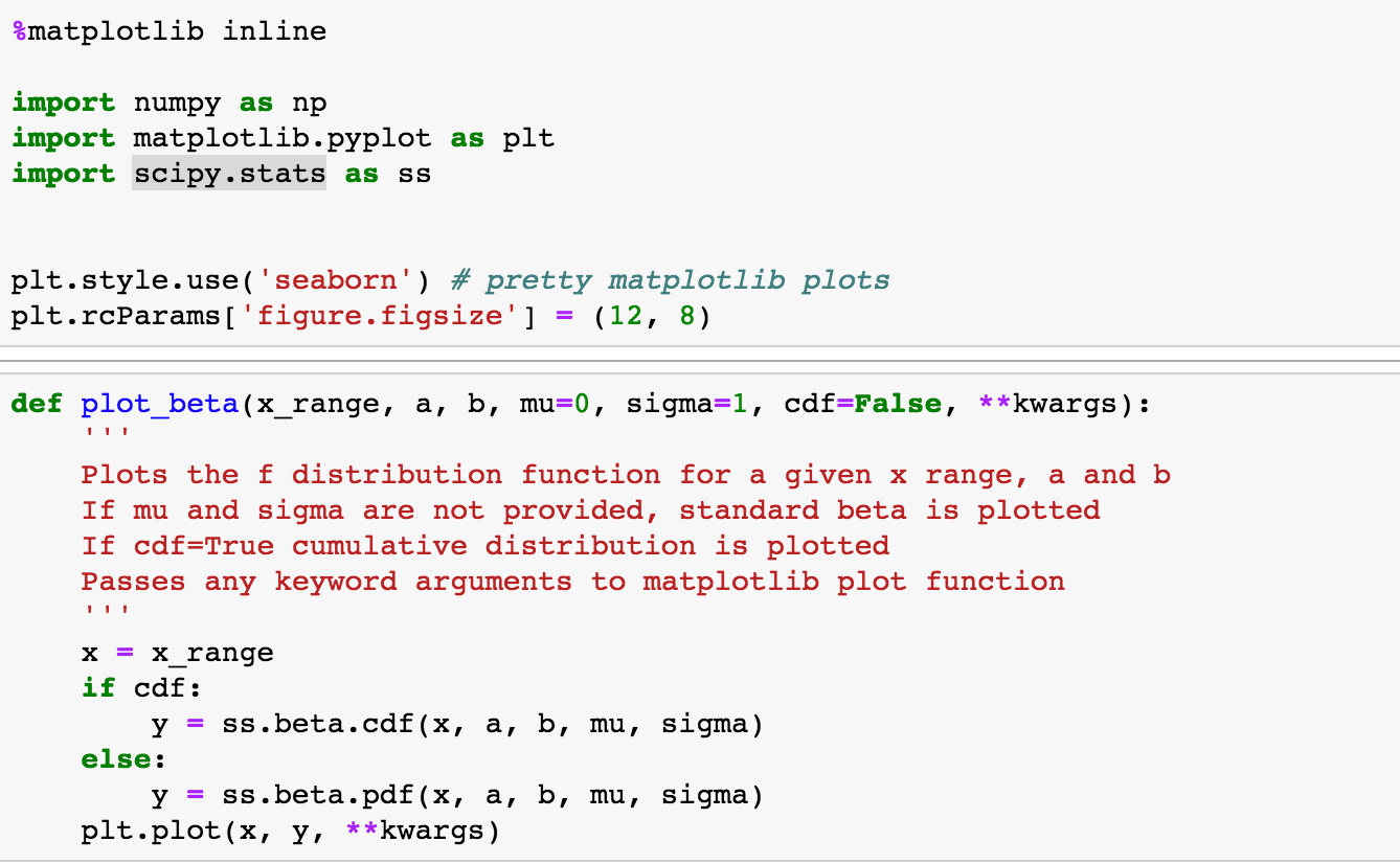
In Python, we have scipy.stats package which contains all most all required distributions cooked for us. Refer to this link for more details.

Lets try out, load all necessary packages.

 

Now, lets take a scenario, you have four books in library, each book is rated by students good(1) or bad(0).

Probability of a book being good using naive method way would be:

#no of good ratings /# no of total ratings(good ratings + bad ratings)

Red Book Probability Being Good=2/2 =1
Blue Book Probability Being Good=8/9
Orange Book Probability Being Good=80/90
Black Book Probability Being Good=700/800

These probabilities can be represented as beta distribution as [0,1].

Peak of each book probability distribution represents the mean which is α±/(α±+α²).

If someone need to choose which Book should I read based on above ratings, one can look of these beta distribution and come up with different choosing criteria.

In general people first look for ratings then also look for no of people rated in scenarios like this so for most the people Black Book (700/800) will be a better choice than Red Book (2/2) this can be easily figured out by checking beta distribution with Best Worst Case Scenario.

 

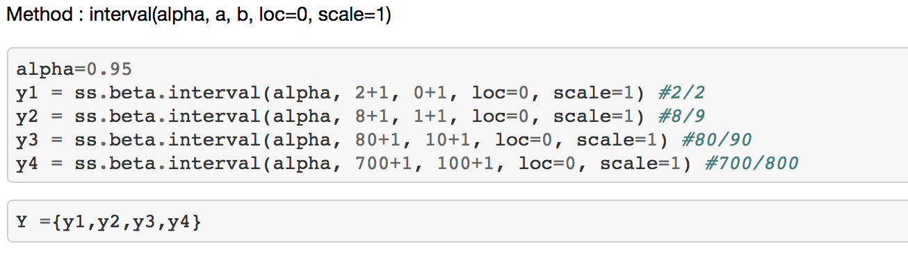
In this case y4's worst case lower bound probability is better than others hence Black Book makes a safe choice for readers (users, who don't want to take risk).

Beta distribution are very well know and widely used in data science. I would love to know more scenarios where you have used Beta distribution in practice.

 
References

• Understanding the beta distribution (using baseball statistics)
• Plotting Distributions with matplotlib and scipy
• Beta distribution
• An intuitive interpretation of the beta distribution

 
Bio: Krishna Kumar Tiwari is a Data Science Architect at InMobi.

Original. Reposted with permission.

Related:

• 5 Probability Distributions Every Data Scientist Should Know
• What is Poisson Distribution?
• How to count Big Data: Probabilistic data structures and algorithms