Get Started with Statistics for Data Science
This article was published as a part of the Data Science Blogathon
What is Statistics?
The Oxford dictionary defines statistics as ‘the practice or science of collecting and analyzing numerical data in large quantities, especially for the purpose of inferring proportions in a whole from those in a representative sample.’
Ben Baumer, author of ‘Modern Data Science with R’ book defines it as “the science of modeling the randomness present in real-world observations.”
In my words, from what I learned, this is the study of collecting and extracting information from quantitative data for making inferences and decisions. The result of analysis from sample information is generalized to the whole population data.
Types:
There are 2 broad categories of statistics:
1) Descriptive statistics
2) Inferential statistics
Descriptive statistics:
These represent the numbers that describe the entire data set. These numbers are like a summary of all the observations in the data. For instance, the average value of a data field is a descriptive statistic.
Descriptive statistics are classified into 5 major types:
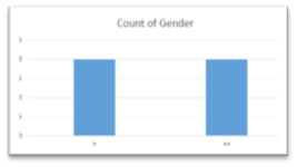
i) Measure of frequency
This indicates the count-related attributes of the data, like the frequency of occurrence, count, and percent values.
ii) Measure of central tendency:
This indicates the central aspect of the data. Mean, median, and mode are the attributes that talk about the central tendency of the data
Input_data = {19,19,23,39,45,48,48,48,67}
Mean (average) : sum of all values/count of all values = 356/9=39.56
Median : middle value in the sorted data = 45
Mode : most occurring value = 48
Data might not always be symmetrical around the center. They may be populated more to the left or right.
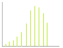
Left skewed data:
More data towards the right end.
Eg – age-wise histogram plot of pension scheme account holders
In the case of left skew, Mean < Median
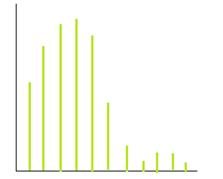
Right skewed data:
More data towards the left end (lower values in magnitude).
Eg – age-wise histogram plot of gaming account holders
In the case of right skew, Mean > Median
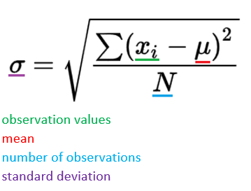
iii) Measure of dispersion:
This indicates the spread out with data. Standard deviation and variance are useful values that explain the spread of the data w.r.t the mean.
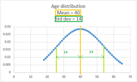
Fig. This is a frequency plot called a histogram. The age values are plotted against the count of occurrences.
Standard deviation is the average difference between the mean and the points in the data.
iv) Measure of position:
This is helpful to describe the values in relation to one another. Percentiles ranks can give insight into the position of a value w.r.t to other values. Unlike standard deviation, this is not affected by the extreme values in the data.
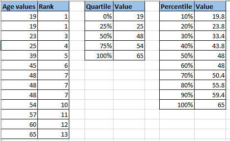
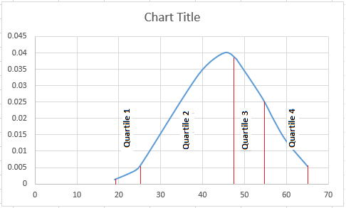
Note – the quartiles are not evenly separated, because the values are not evenly spread
In real scenarios, the data might not be exactly evenly distributed, ie it can be skewed data. There can be more values towards the left end(lower values) or towards the right end(higher values).
The main characteristic of these kinds of data is the mean and median will not be the same. So the data will be skewed.
v) Measures of association:
It is important to identify the relationship between variables.
Covariance
Covariance is a measure of the relation between two variables. The direction of the result indicates the type of relation between the two variables. A positive result indicates that they are directly proportional, while a negative result indicates they are inversely proportional. The result of the covariance will change when the unit of the variables, the area of a house (sqft, etc), or the currency (INR, USD, etc) vary. Covariance value can range from -infinity to +infinity.
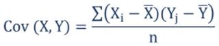
Covariance of 2 variables X and Y is defined as the product of each of its observations with the difference from their mean.
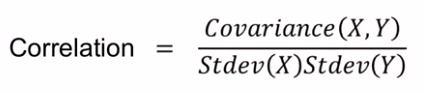
Correlation
Correlation is a measure of how strongly two variables are related to each other. Correlation is not affected by the scale of the variables. It just mentions the strength of the relation between the variables.
While covariance only identifies if it is a positive or a negative relationship, correlation establishes both the direction (positive or negative) and strength of the relation between the two variables. Covariance cannot help to identify the strength of the relationship, as its values are affected by the unit of the two variables.
Pearson correlation coefficient value ranges from -1 to +1. Values nearer to +/-1 indicates strong relation, while values near to 0 indicate a weak relationship
-1 – indicates that the two variables are inversely coupled strongly ie., when one increases, the other decreases, like marks and rank.
0 – indicates no relation between them or in other words, they are uncorrelated, like wind speed and student mark.
+1 – indicates a strong positive correlation ie., when one increases, the other also increases, like sqft area of the house and house price
Generally, as the correlation value is not affected by the unit of the two variables and it can ascertain the strength of the relationship, and it is preferred over covariance.
Some sample python code to calculate the aforementioned values:
import pandas as pd
import statistics
import numpy as np
data = [['fred', 20, 90], ['ron', 18, 85], ['bill', 28, 95], ['george',20, 89]]
# Create the pandas DataFrame
df = pd.DataFrame(data, columns = ['Name', 'Age', 'Mark'])
print('Count',len(df))
print('Mean',statistics.mean(df['Age']))
print('Median',statistics.median(df['Age']))
print('Mode',statistics.mode(df['Age']))
print('Std',statistics.stdev(df['Age']))
print('Variance',statistics.variance(df['Age']))
print('Covariance',df.cov())
print('Correlation',df.corr())
Output:
Count 4
Mean 21.5
Median 20.0
Mode 20
Std 4.43471156521669
Variance 19.666666666666668
Covariance Age Mark
Age 19.666667 17.166667
Mark 17.166667 16.916667
Correlation Age Mark
Age 1.000000 0.941159
Mark 0.941159 1.000000
Distributions
Distributions play a key role in understanding the data. Distributions are the frequency plot of all values for a variable in the data. The distributions are used to calculate the probability of values, based on the spread of the data. The function describing the probability of the values is called the probability density/mass function.
Based on the properties of the data and the spread, there are different types of distributions. Every distribution has a density function for finding probabilities.
Key differentiating points:
1) Data – discrete data(whole numbers with limited values, like months or gender) or continuous data(numbers that can take any value, like temperature, height)
2) Skewedness – distribution can be symmetric or skewed
3) Boundaries – the values can have strict lower or upper boundaries (like a mark cannot exceed 100)
4) Outliers or tail values – the extreme values of the data (usually outliers) can be rare or common
5) Number of modes – mode is the most frequently occurring value in the data. In case there is more than one most recurring value, then it might mean that there is more than one population in the data. The populations have to be separated and dealt with.
Density functions:
i) Probability mass function(PMF):
PMF also known as the discrete density function, is a density function for discrete data. This density function is used to calculate the probability of a certain value of a discrete random variable.
P(X=x) = f(x)
X = random variable
x = one possible value of variable X
The probability value is always a non-negative number. The sum of the probability of all possible values of X will equal 1.
Example:
A fair coin is tossed twice. Let us consider we want to identify the probability that the result has one head. When two coins are tossed, the resultant values can be {HH, HT, TH, TT}.
Let us consider X as the random variable with the count of heads resulted from a coin toss.
X can have {0,1,2}.
We need P(X=1) = P({HT,TH})= number of outcomes with {HT,TH}/total number of outcomes = 2.4 = 0.5
Also, the sum of probability of all values of X will equal 1:
P(X=0) + P(X=1) + P(X=2)
=cnt({TT})/ cnt({HH, HT, TH, TT}) + cnt({HT,TH})/cnt({HH, HT, TH, TT}) + cnt({HH})/cnt({HH, HT, TH, TT})
=1/4 + 2/4 + 1/4
=1
ii) Probability Density Function(PDF):
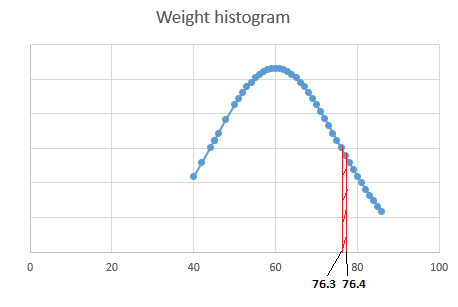
For continuous variables, p(X=x) = 0, for all x∈R
P(weight = 76.34kg)=0, as it can be argued that weight 76.3!=76.34 and 76.341!=76.34
Hence it will be more appropriate to use P(weight between 76.3 to 76.4) for continuous variables. So instead of calculating the probability of the variable being a particular single value, the probability is calculated for the variable to be within a range of values.
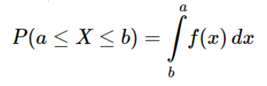
The area between the limit values a and b in the function f(x) is calculated by using integration.
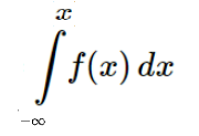
iii) Cumulative distribution function(CDF):
The cumulative density function calculates the probability that a random variable X takes a value less than equal to a particular value x. As this does not calculate for a particular value, this function is applicable for both discrete and continuous variables.
P(X≤x) = f(x), for all x∈R
This can also be written as,
Example:
When tolling a fair die, every outcome has an equal probability of 1/6.
For PMF, we use P(X=x), for all x P(X)=1/6
In the case of CDF, P(X<=x) calculates the cumulative probabilities of all values of X that is before x and x. P(X=1)=1/6, P(X=2)=2/6, P(X=3)=3/6, etc.,
Python library to runt hese functions;
from scipy.stats import norm
norm.pdf(0.01), norm.cdf(0.01)
Types of distributions:
Some of the common distributions are explained here.
1) Uniform distribution:
The uniform distribution indicates that all of a variable’s outcomes are equally probable or that the probability is uniformly distributed.
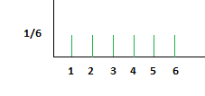
Fig. rolling fair die results in uniform distribution
2) Binomial distribution:
This is a distribution well suited for discrete data.
A Bernoulli trial is an experiment that can have exactly two possible outcomes – success and failure. These outcomes are mutually exclusive.
The binomial distribution is the repetition of the Bernoulli trial when the probabilities of the outcomes are maintained the same for every trial. This means the Bernoulli trials are independent trials.
For example, consider a card is drawn from a deck of playing cards. To keep the probabilities the same, during the next draw, the drawn card is placed back in the deck.
The PMF, P(x) = nCr · pr (1 − p)n−r
n- total number of trials
p-probability of success in a single Bernoulli trial
r-total number of successful trials, for which we are calculating the probability.
nCr – number of combinations (formula=[n!/r!(n−r)!])
Example – If there are 4 trails from a deck of playing cards with replacement, what is the probability of getting exactly 2 hearts.
p=1/4
n=4
r=2
On substitution of the variables, P(x) = 0.21
3) Gaussian distribution:
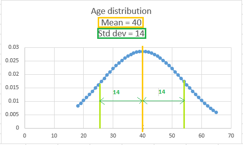
Also known as the normal distribution, this is the most commonly used type of distribution observed in real data. It has a bell-shaped curve and is assumed to be symmetrical around the mean value. The bell shape is because the data values near the mean are more frequent than the ones far away from the mean.
The normal distribution is for continuous data and can be used for discrete data as well
Example of a Gaussian distribution data – marks scored by students in an exam. More students would have secured average marks, while there will be a few exceptional performers and a few underperformers.
Sample representation:
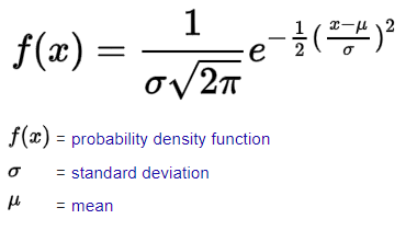
Formula for PDF:
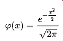
Standard normal distribution (z-distribution):
When the normal distribution has a mean=0 and standard deviation=1, then it is called the standard normal distribution.
Here the formula gets simplified on substitution too,
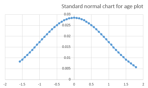
When the normal distribution data is converted to a standard normal distribution, it aids in comparing different datasets with different means and standard deviations.
The before and after mean values are distinguished by +/- signs.
The data points on the distribution are no longer the actual data points x, but the z-score of the actual data points.
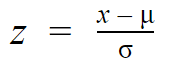
This Z-score aids in decision-making processes, especially in the study of outliers in the data.
4) Poisson distribution:
This is again a distribution suitable for discrete data. This distribution helps us to get the probability for a given number of events to occur within a fixed period of time.
Example – number of customers visiting a shop to purchase product A every week, which can help the shopkeeper to stock product A accordingly.
PMF is given by,
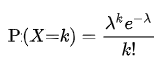
λ – average event occurrence (say 50 customers per week)
k – number of events for which probability is calculated (number of customers for which probability is calculated)
Inferential statistics:
Inferential statistics are generally used to infer details from the sample data, to make decisions for the actual population data.
Here, population – refers to the entire set of real data and sample data – refers to the considerably less volume of the data to which we have access for analysis.
This is a very broad area, and we cannot do it justice in this blog.
Endnote:
This content covers the basics of Statistics, mainly elaborating the Descriptive type and distributions.
Real learning comes by using the knowledge learned by providing a solution in actual data.
The media shown in this article are not owned by Analytics Vidhya and are used at the Author’s discretion.


