Rapid-Fire EDA Process Using Python for ML Implementation

Introduction

In the field of machine learning (ML), the effectiveness and accuracy of any model heavily depend on the quality of the data it’s trained on, emphasizing the critical importance of Exploratory Data Analysis (EDA). With Python and its powerful libraries like Pandas, NumPy, and Matplotlib, EDA can now be conducted with unprecedented efficiency. In this article, we explore a “Rapid-Fire EDA Process” that leverages Python’s capabilities to swiftly explore and preprocess datasets for ML implementation.

Through practical examples and code snippets, we aim to empower readers with the knowledge and techniques necessary to accelerate their EDA workflow and pave the way for successful ML implementations.

Learning Objectives:

• Understand how a machine learning process works.
• Understand what Exploratory Data Analysis (EDA) is.
• Learn to perform the rapid-fire EDA process using Python.

This article was published as a part of the Data Science Blogathon.

Understanding ML Best Practices and Project Roadmap

When a customer wants to implement ML(Machine Learning) for the identified business problem(s) after multiple discussions along with the following stakeholders from both sides – Business, Architect, Infrastructure, Operations, and others. This is quite normal for any new product/application development. 

But in the ML world, this is quite different. because, for new application development, we have to have a set of requirements in the form of sprint plans or traditional SDLC form and it depends on the customer for the next release plan.

But in ML implementation, as a Data Scientist, we need to initiate the below activity first.

Data Source Identification and Data Collection

• Organization’s key application(s) – it would be internal or external applications or websites
• It would be streaming data from the web (Twitter/Facebook – any Social media)

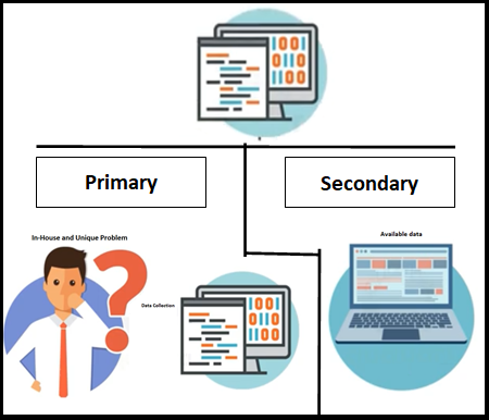
Once you’re comfortable with the available data, you can start work on the rest of the machine learning process model. 

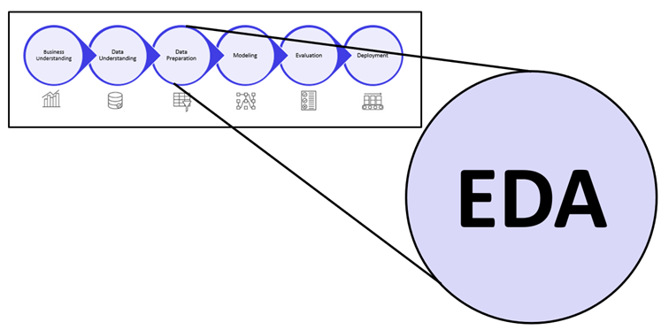
The Machine Learning Process

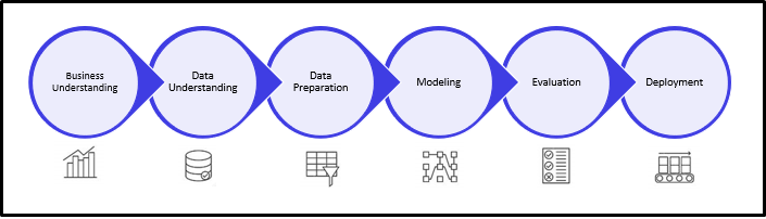
Let’s jump into the EDA process, which is the third step in the above picture. In the data preparation, EDA gets most of the effort and unavoidable steps. Let’s dive into the details of this.

What is Exploratory Data Analysis (EDA)?

Exploratory Data Analysis is an unavoidable step in fine-tuning a given data set(s). It is a different form of analysis to understand the insights of the key characteristics of various entities of the data set like column(s), row(s). It is done by applying Pandas, NumPy, statistical methods, and data visualization packages. 

The outcomes of this phase are as follows:

• Better understanding of the given dataset which helps clean up the data.
• It gives you a clear picture of the features and the relationships between the data.
• Providing guidelines for essential variables and leaving behind/removing non-essential variables.
• Handling missing values or human error.
• Identifying outliers.
• The EDA process would maximize insights into a dataset.
• It is also helpful when applying machine learning algorithms later on.

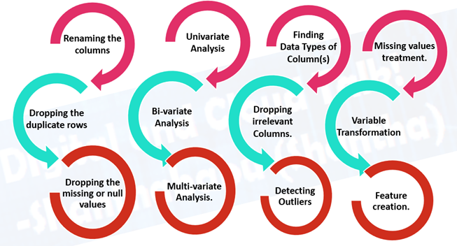
This process is time-consuming but very effective, the below activities are involved during this phase, it would be varied and depends on the available data and acceptance from the customer.

Rapid-Fire EDA Process Using Python

Now that you have some idea, let’s implement all these using the Automobile – Predictive Analysis dataset.

Step 1: Import Key Packages

Let’s first import all the important functions from the sklearn library.

print("######################################")
print("       Import Key Packages            ")
print("######################################")
import pandas as pd
import numpy as np
import matplotlib.pyplot as plt
import seaborn as sns
from IPython.display import display
import statsmodels as sm
from statsmodels.stats.outliers_influence import variance_inflation_factor
from sklearn.model_selection import train_test_split,GridSearchCV,RandomizedSearchCV
from sklearn.linear_model import LinearRegression,Ridge,Lasso
from sklearn.tree import DecisionTreeRegressor
from sklearn.ensemble import RandomForestRegressor,GradientBoostingRegressor
from sklearn.metrics import r2_score,mean_squared_error
from sklearn import preprocessing

######################################
Import Key Packages
######################################

Step 2: Load .csv Files

Let’s first load the dataset into a pandas dataframe before we jump onto performing the analysis.

df_cars = pd.read_csv('./cars.csv')

Step 3: Get the Dataset Information

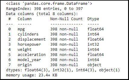
print("############################################")
print("          Info Of the Data Set")
print("############################################")
df_cars.info()

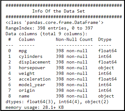
Observation:

• We could see that the features/column/fields and their data type, along with Null count.
• The name feature is an object type in the given data set.

Let go and see the given data set file and perform some EDA techniques on them.

Step 4: Data Cleaning/Wrangling

The process of cleaning and unifying messy and complex data sets for easy access and analysis.

Action:

• replace(‘?’,’NaN’)
• Converting “horsepower” Object type into int

df_cars.horsepower = df_cars.horsepower.str.replace('?','NaN').astype(float)
df_cars.horsepower.fillna(df_cars.horsepower.mean(),inplace=True)
df_cars.horsepower = df_cars.horsepower.astype(int)
print("######################################################################")
print("          After Cleaning and type covertion in the Data Set")
print("######################################################################")
df_cars.info()

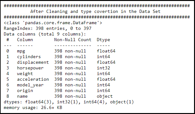
Observation:

• We could see that the features/column/fields and their data type, along with Null count.
• Horsepower is now int type.
• Name still as an object type in the given data set, since we’re going to drop it during the EDA phase.

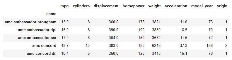
Step 5: Grouping Them by Names

• Correcting the brand name (Since misspelled, we have to correct it)

df_cars['name'] = df_cars['name'].str.replace('chevroelt|chevrolet|chevy','chevrolet')
df_cars['name'] = df_cars['name'].str.replace('maxda|mazda','mazda')
df_cars['name'] = df_cars['name'].str.replace('mercedes|mercedes-benz|mercedes benz','mercedes')
df_cars['name'] = df_cars['name'].str.replace('toyota|toyouta','toyota')
df_cars['name'] = df_cars['name'].str.replace('vokswagen|volkswagen|vw','volkswagen')
df_cars.groupby(['name']).sum().head()

After correcting the names:

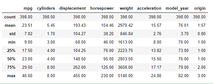
Step 6: Summary of Statistics

Now we can check the summary statistics like mean, standard deviation, percentiles, etc.

display(df_cars.describe().round(2))

Step 7: Dealing with Missing Values

Fill in the missing data points of horsepower by mean of horsepower value.

meanhp = df_cars['horsepower'].mean()
df_cars['horsepower'] = df_cars['horsepower'].fillna(meanhp)

Step 8: Skewness and Kurtosis

Finding the Skewness and Kurtosis of mpg feature:

print("Skewness: %f" %df_cars['mpg'].skew())
print("Kurtosis: %f" %df_cars['mpg'].kurt())

The skewness and kurtosis values turn out to be the following:

Skewness: 0.457066
Kurtosis: -0.510781

Step 9: Categorical Variable Move

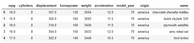
If you look at the dataset carefully, you will notice that the ‘origin’ feature is not actually a continuous variable but a categorical variable. So we need to treat such variables in a different way. There are several ways of doing that. What we are going to do here is replace the categorical variable with actual values.

df_cars['origin'] = df_cars['origin'].replace({1: 'america', 2: 'europe', 3: 'asia'})
df_cars.head()

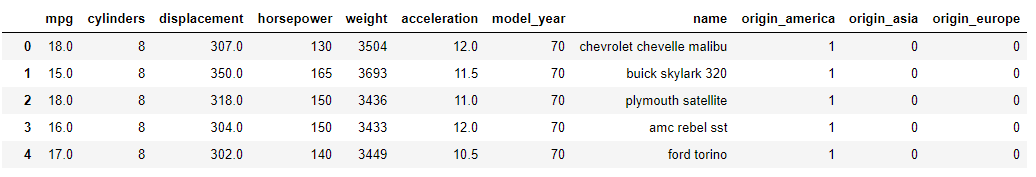
Step 10: Creating Dummy Variables

Values like ‘america’ cannot be read into an equation. So we create 3 simple true or false columns with titles equivalent to “Is this car America?”, “Is this care European?” and “Is this car Asian?”. These will be used as independent variables without imposing any kind of ordering between the three regions. Let’s apply the below code.

cData = pd.get_dummies(df_cars, columns=['origin'])
cData

Step 11: Removing Columns 

For this analysis, we won’t be needing the car name feature, so we can drop it.

df_cars = df_cars.drop('name',axis=1)

Step 12: Conducting the Analysis

There are 3 types of data analysis: univariate, bivariate, and multivariate. Let’s explore them one by one.

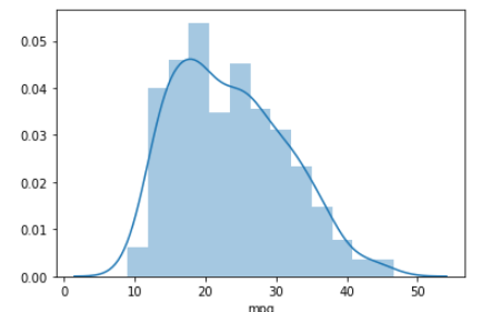
1. Univariate Analysis:

“Uni” +“Variate” = Univariate, meaning one variable or feature analysis. The univariate analysis basically tells us how data in each feature is distributed. just sample as below.

sns_plot = sns.distplot(df_cars["mpg"])

2. Bivariate Analysis:

“Bi” +“Variate” = Bi-variate, means two variables or features are analyzed together, to find out how they are related to each other. Generally, we use it to find the relationship between the dependent and independent variables. Even you can perform this with any two variables/features in the given dataset to understand how they are related to each other.

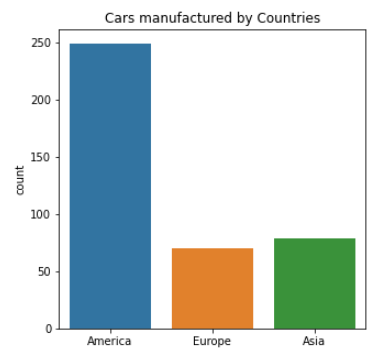
Here we will be plotting a bar plot to depict the count of cars manufactured by each country. Since this is a categorical data, we are plotting it on a bar plot.

fig, ax = plt.subplots(figsize = (5, 5))
sns.countplot(x = df_cars.origin.values, data=df_cars)
labels = [item.get_text() for item in ax.get_xticklabels()]
labels[0] = 'America'
labels[1] = 'Europe'
labels[2] = 'Asia'
ax.set_xticklabels(labels)
ax.set_title("Cars manufactured by Countries")
plt.show()

# Exploring the range and distribution of numerical Variables
fig, ax = plt.subplots(6, 2, figsize = (15, 13))
sns.boxplot(x= df_cars["mpg"], ax = ax[0,0])
sns.distplot(df_cars['mpg'], ax = ax[0,1])
sns.boxplot(x= df_cars["cylinders"], ax = ax[1,0])
sns.distplot(df_cars['cylinders'], ax = ax[1,1])
sns.boxplot(x= df_cars["displacement"], ax = ax[2,0])
sns.distplot(df_cars['displacement'], ax = ax[2,1])
sns.boxplot(x= df_cars["horsepower"], ax = ax[3,0])
sns.distplot(df_cars['horsepower'], ax = ax[3,1])
sns.boxplot(x= df_cars["weight"], ax = ax[4,0])
sns.distplot(df_cars['weight'], ax = ax[4,1])
sns.boxplot(x= df_cars["acceleration"], ax = ax[5,0])
sns.distplot(df_cars['acceleration'], ax = ax[5,1])
plt.tight_layout()

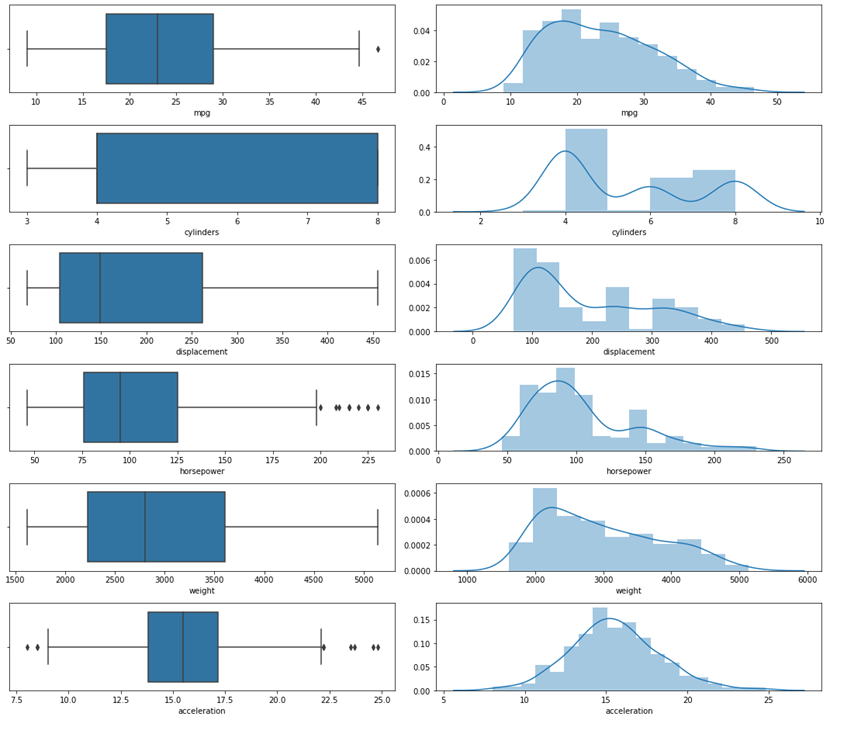
Plot Numerical Variables

plt.figure(1)
f,axarr = plt.subplots(4,2, figsize=(10,10))
mpgval = df_cars.mpg.values
axarr[0,0].scatter(df_cars.cylinders.values, mpgval)
axarr[0,0].set_title('Cylinders')
axarr[0,1].scatter(df_cars.displacement.values, mpgval)
axarr[0,1].set_title('Displacement')
axarr[1,0].scatter(df_cars.horsepower.values, mpgval)
axarr[1,0].set_title('Horsepower')
axarr[1,1].scatter(df_cars.weight.values, mpgval)
axarr[1,1].set_title('Weight')
axarr[2,0].scatter(df_cars.acceleration.values, mpgval)
axarr[2,0].set_title('Acceleration')
axarr[2,1].scatter(df_cars["model_year"].values, mpgval)
axarr[2,1].set_title('Model Year')
axarr[3,0].scatter(df_cars.origin.values, mpgval)
axarr[3,0].set_title('Country Mpg')
# Rename x axis label as USA, Europe and Japan
axarr[3,0].set_xticks([1,2,3])
axarr[3,0].set_xticklabels(["USA","Europe","Asia"])
# Remove the blank plot from the subplots
axarr[3,1].axis("off")
f.text(-0.01, 0.5, 'Mpg', va='center', rotation='vertical', fontsize = 12)
plt.tight_layout()
plt.show()

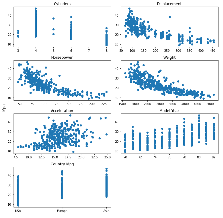
Observation:

So let’s find out more information from these 7 charts

• Well, nobody manufactures 7 cylinders. (Why…Does anyone know?)
• 4 cylinder has better mileage performance than other and most manufactured ones.
• 8 cylinder engines have a low mileage count… of course, they focus more on pickup (fast cars).
• 5 cylinders, performance-wise, compete none neither 4 cylinders nor 6 cylinders.
• Displacement, weight, and horsepower are inversely related to mileage.
• More horsepower means low mileage.
• Year-on-year, manufacturers have focussed on increasing the mileage of the engines.
• Cars manufactured in Japan majorly focus more on mileage.

3. Multi-Variate Analysis:

Multi-variate analysis means analyzing more than two variables or features together, to know how they relate to each other.

sns.set(rc={'figure.figsize':(11.7,8.27)})
cData_attr = df_cars.iloc[:, 0:7]
sns.pairplot(cData_attr, diag_kind='kde')   
# to plot density curve instead of the histogram on the diagram # Kernel density estimation(kde)

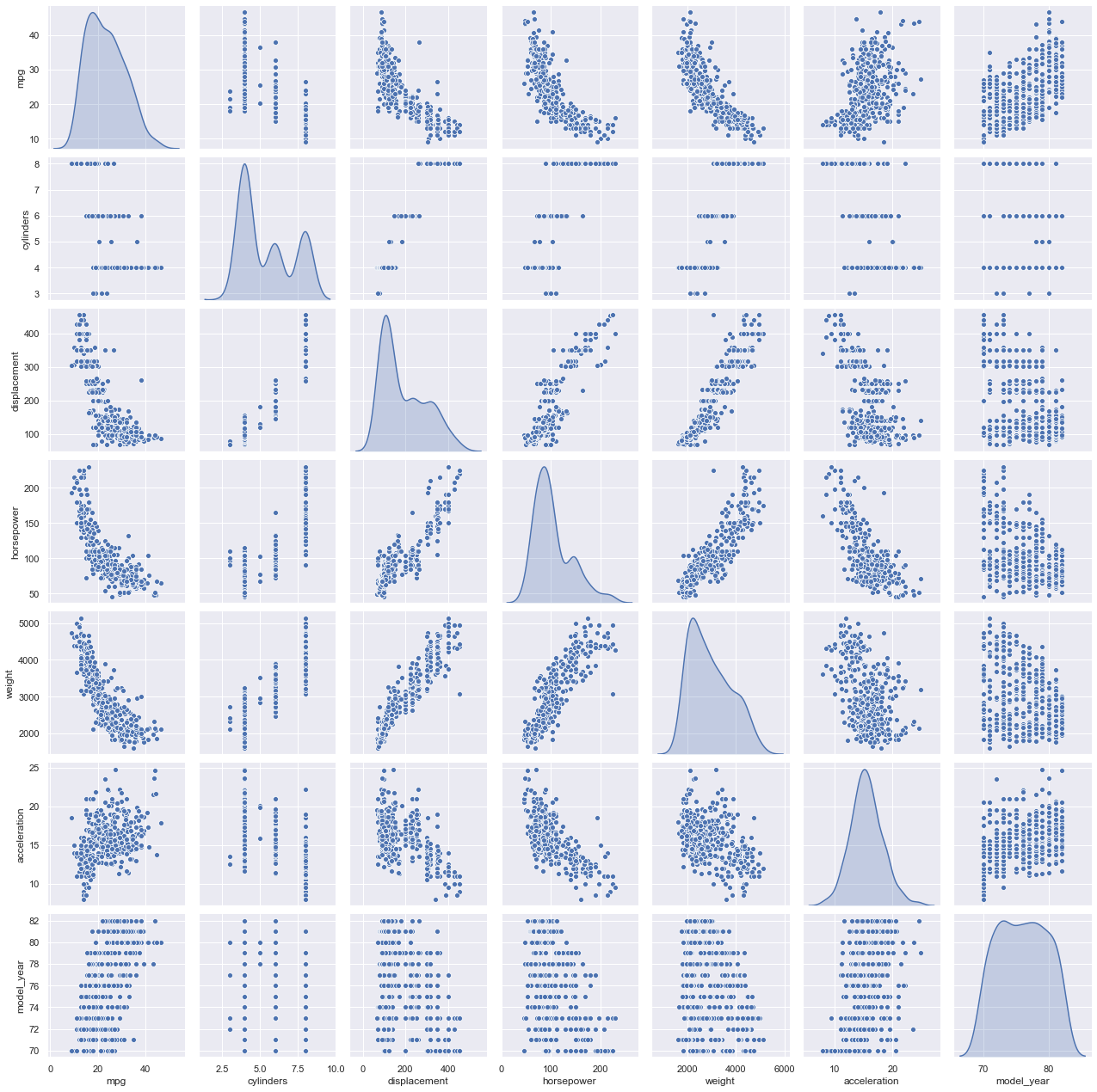
Observation:

• Between ‘mpg’ and other attributes indicates the relationship is not really linear. 
• However, the plots also indicate that linearity would still capture quite a bit of useful information/pattern. 
• Several assumptions of classical linear regression seem to be violated, including the assumption of no heteroscedasticity.

Step 13: Distributions of the Variables/Features

df_cars.hist(figsize=(12,8),bins=20)
plt.show()

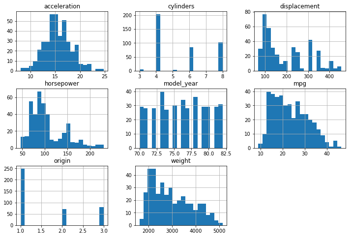
Observation:

• The acceleration of the cars in the data is normally distributed and most of the cars have an acceleration of 15 meters per second squared.
• Half of the total number of cars (51.3%) in the data has 4 cylinders.
• Our output/dependent variable (mpg) is slightly skewed to the right.

Let’s visualize the distribution of the features of the cars now.

Step 14: Finding Correlation

We use a heatmap to find the relationship between different features.

How to read it? Very simple:

• Dark color represents a positive correlation,
• Light color/ white is a towards the negative correlation.

plt.figure(figsize=(10,6))
sns.heatmap(df_cars.corr(),cmap=plt.cm.Reds,annot=True)
plt.title('Heatmap displaying the relationship betweennthe features of the data',
         fontsize=13)
plt.show()

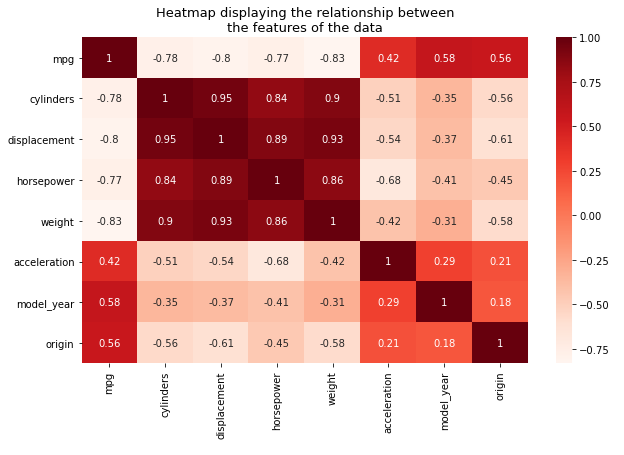
Relationship between the Miles Per Gallon (mpg) and the other features:

• We can see that there is a relationship between the mpg variable and the other variables and this satisfies the first assumption of linear regression.
• Strong Negative correlation between displacement, horsepower, weight, and cylinders.
  • This implies that, as any one of those variables increases, the mpg decreases.
• Strong Positive correlations between the displacement, horsepower, weight, and cylinders.
  • This violates the non-multicollinearity assumption of Linear regression.
  • Multicollinearity hinders the performance and accuracy of our regression model. To avoid this, we have to get rid of some of these variables by doing feature selection.
• The other variables, i.e., acceleration, model, and origin, are NOT highly correlated with each other.

Conclusion

I trust you were able to fully understand the EDA process through this guide. However, there are many more functions in it. If you’re doing the EDA process clearly and precisely, there is a 99% guarantee that you could build your model selection, hyperparameter tuning, and deployment process effectively without further data cleaning. You have to continuously monitor the data and ensure the model output is sustainable, to predict, classify, or cluster it.

Key Takeaways:

• Exploratory Data Analysis (EDA) is a form of analysis to understand the insights of the key characteristics of various entities of a given dataset like column(s), row(s), etc.
• It is done by applying Pandas, NumPy, statistical methods, and data visualization packages.
• The 3 types of data analysis involved in EDA are univariate, bivariate, and multivariate.

Frequently Asked Questions

The media shown in this article is not owned by Analytics Vidhya and is used at the Author’s discretion.

Shanthababu Pandian 21 Feb 2024