Step-by-Step guide for Image Classification on Custom Datasets
This article was published as a part of the Data Science Blogathon
Agenda
- Introduction
- Why is learning image classification on custom datasets significant?
- Steps to develop an image classifier for a custom dataset
- Summary
Introduction
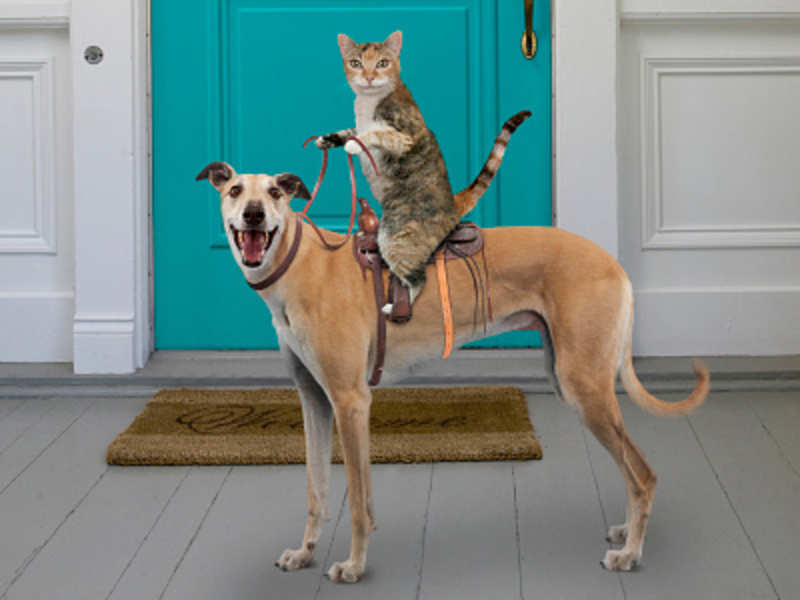
Image taken from source
Cats or dogs-Phew!Don’t worry, readers. I won’t bore you with this dataset. We must all be tired of learning how to perform image classification using such habitual datasets. So, I have something more interesting in store for you.

Image taken from source
In this blog, I will be discussing how to classify among the images of hand gestures of rock, paper, and scissors using a VGG-19 model trained on the rock-paper-scissors Kaggle dataset. To be precise, given the image of one of these hand gestures, the model classifies if it is that of a rock, paper, or scissors.VGG-19 is one of the pre-trained Convolutional Neural Networks(CNNs) and is 19 layers deep! Just like other transfer learning models, it is trained on 1000 categories. Every time we use it to classify a problem, we should customize the last layer of the model according to the number of classes of our problem. I will elaborate practically on this when we proceed to the section of building our model.
Why is learning image classification on custom datasets significant?
Many a time, we will have to classify images of a given custom dataset. To be precise, in the case of a custom dataset, the images of our dataset are neatly organized in folders. It can either be collected manually or downloaded directly from common sites for datasets such as Kaggle. When we use Tensorflow or Keras datasets, we easily obtain the values of x_train,y_train,x_test, and y_test while loading the dataset itself. These values are significant for understanding how our training and validation datasets’ labels are encoded and obtain the classification report and the confusion matrix. But, how can we manage to derive these values for our custom dataset? How do we build an efficient image classifier using the dataset available to us in this manner?
Steps to develop an image classifier for a
custom dataset
Step-1: Collecting your dataset
Step-2: Pre-processing of the images
Step-3: Model training
Step-4: Model evaluation
Step-1: Collecting your dataset
Let’s download the dataset from here. The dataset consists of 2188 color images of hand gestures of rock, paper, and scissors. The distribution of the hand gesture images among the three categories are as follows:
| Category | No. of images |
| Rock | 726 |
| Paper | 710 |
| Scissors | 752 |
Further, I divided the dataset into a train-test-Val split in 80-20 split ratio as described below:
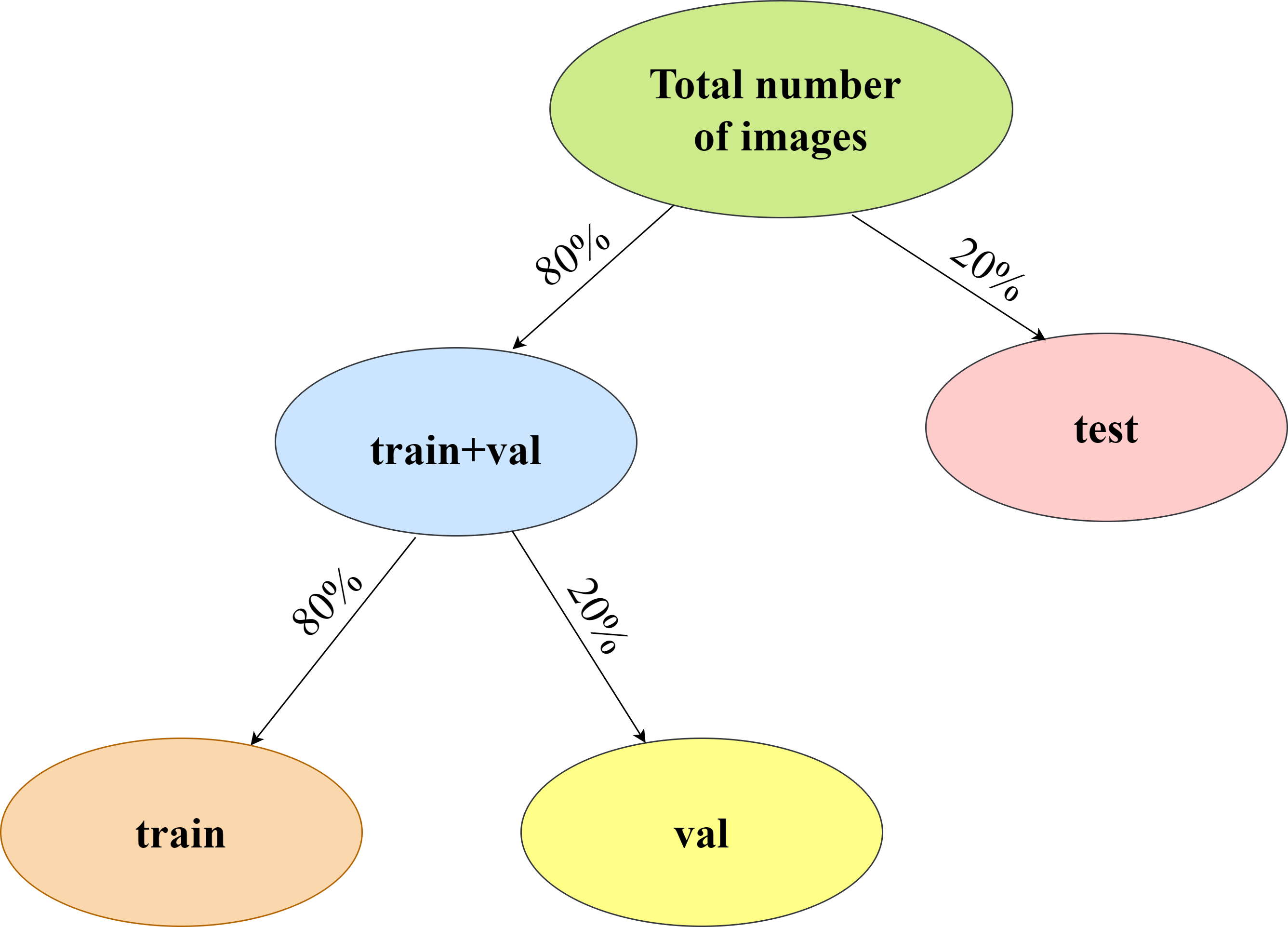
| Category | Total number of images (T) |
No. of training images (0.8*0.8*T) |
No. of validation images (0.2*0.8*T) |
No. of testing images (0.2*T) |
| Rock | 726 | 465 | 116 | 145 |
| Paper | 710 | 456 | 114 | 142 |
| Scissors | 752 | 480 | 120 | 150 |
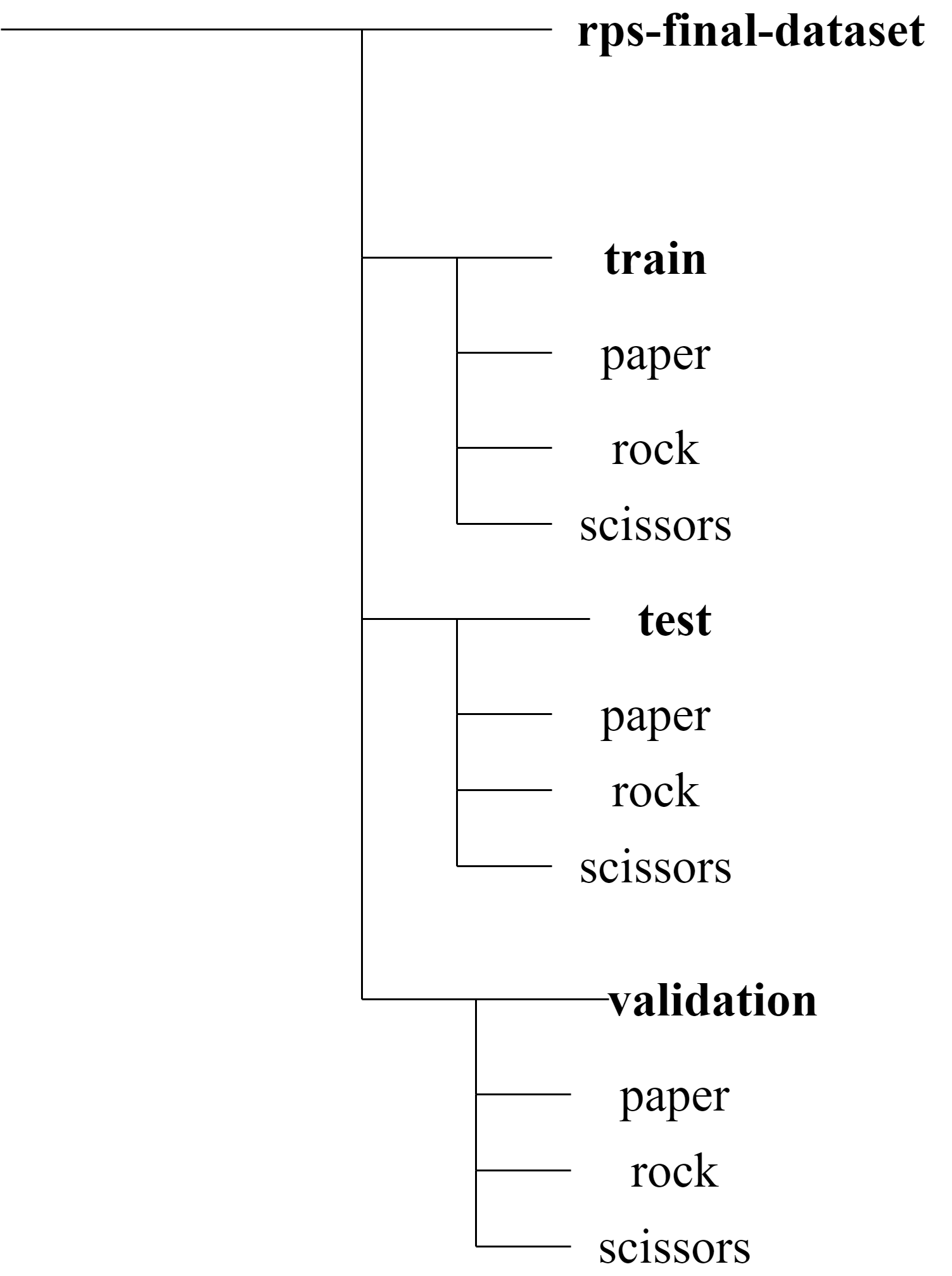
The above is the illustration of the folder structure. The training dataset folder named “train” consists of images to train the model. The validation dataset folder named “val”(but it is shown as validation in the above diagram only for clarity. Everywhere in the code, val refers to this validation dataset) consists of images to validate the model in every epoch. They are used to obtain the training and validation accuracies and losses in every epoch while training the model. The images of the folder named “test” are completely unseen images of the hand gestures.
The performance of our model on the testing dataset shows how accurate our model is.
Step-2: Pre-processing of the images
We will be training a VGG-19 model on our custom training dataset to classify among the three categories-rock, paper, and scissors. The pre-trained CNN model inputs a color image of dimensions 224×224 of one of the three hand gestures. However, all the images of the dataset are of dimensions 300×200. Hence, they must all be resized to the required dimension.
While resizing the images, let us also derive x_train,x_test,x_val,y_train,y_test and y_val hand-in-hand. These terms can be described in a nutshell as follows:
x_train: Numpy arrays of the images of the training dataset
y_train: Labels of the training dataset
x_test: Numpy arrays of the images of the testing dataset
y_test: Labels of the testing dataset
x_val: Numpy arrays of the images of the validation dataset
y_val: Labels of the validation dataset
Firstly, let us import the required packages:
from tensorflow.keras.layers import Input, Lambda, Dense, Flatten,Dropout
from tensorflow.keras.models import Model
from tensorflow.keras.applications.vgg19 import VGG19
from tensorflow.keras.applications.vgg19 import preprocess_input
from tensorflow.keras.preprocessing import image
from tensorflow.keras.preprocessing.image import ImageDataGenerator
from tensorflow.keras.models import Sequential
import numpy as np
import pandas as pd
import os
import cv2
import matplotlib.pyplot as plt
Now, let us proceed to the code and thus compute the above values.
train_path="rps-final-dataset/train"
test_path="rps-final-dataset/test"
val_path="rps-final-dataset/val"
x_train=[]

for folder in os.listdir(train_path):

    sub_path=train_path+"/"+folder

    for img in os.listdir(sub_path):

        image_path=sub_path+"/"+img

        img_arr=cv2.imread(image_path)

        img_arr=cv2.resize(img_arr,(224,224))

        x_train.append(img_arr)

x_test=[]

for folder in os.listdir(test_path):

    sub_path=test_path+"/"+folder

    for img in os.listdir(sub_path):

        image_path=sub_path+"/"+img

        img_arr=cv2.imread(image_path)

        img_arr=cv2.resize(img_arr,(224,224))

        x_test.append(img_arr)

x_val=[]

for folder in os.listdir(val_path):

    sub_path=val_path+"/"+folder

    for img in os.listdir(sub_path):

        image_path=sub_path+"/"+img

        img_arr=cv2.imread(image_path)

        img_arr=cv2.resize(img_arr,(224,224))

        x_val.append(img_arr)
Now, x_train,x_test, and x_val must be divided by 255.0 for normalization.
train_x=np.array(x_train)
test_x=np.array(x_test)
val_x=np.array(x_val)
train_x=train_x/255.0
test_x=test_x/255.0
val_x=val_x/255.0
At last, let us compute the labels of the corresponding datasets using ImageDataGenerator.This is used because our images are stored in folders. We must walk through the folders and find out the corresponding labels of the images stored here.
Labels in this case are nothing but rock, paper, and scissors.
train_datagen = ImageDataGenerator(rescale = 1./255)
test_datagen = ImageDataGenerator(rescale = 1./255)
val_datagen = ImageDataGenerator(rescale = 1./255)
training_set = train_datagen.flow_from_directory(train_path,
                                                 target_size = (224, 224),
                                                 batch_size = 32,
                                                 class_mode = 'sparse')
test_set = test_datagen.flow_from_directory(test_path,
                                            target_size = (224, 224),
                                            batch_size = 32,
                                            class_mode = 'sparse')
val_set = val_datagen.flow_from_directory(val_path,
                                            target_size = (224, 224),
                                            batch_size = 32,
                                            class_mode = 'sparse')
It can be clearly noted that out of 2188 images,1401 images are used to train our model while 437 images are completely unseen and hence are used to test our model and 350 images are used to validate our model during the training.
train_y=training_set.classes
test_y=test_set.classes
val_y=val_set.classes
We must also understand how the classes have been encoded to interpret classification reports and confusion matrix later. To do this:
training_set.class_indices
train_y.shape,test_y.shape,val_y.shape
We see that y_train,y_val, and y_test are one-dimensional arrays which imply that the labels are NOT one-hot encoded.
If labels were one-hot encoded, these values would have been two-dimensional arrays.
Observing these shapes is essential to decide the appropriate loss function. We will be revisiting the concept in the very next step.
Step-3: Model training
This step includes model building, model compilation, and finally fitting the model.
Step-3.1: Model Building
As mentioned earlier, we will be using the VGG-19 pre-trained model to classify rock, paper, and scissors. Thus, we are dealing with a multi-class classification problem with three categories-rock, paper, and scissors.
Coming to the implementation, let us first import VGG-19:
vgg = VGG19(input_shape=IMAGE_SIZE + [3], weights='imagenet', include_top=False)
#do not train the pre-trained layers of VGG-19
for layer in vgg.layers:
    layer.trainable = False
Now, to customize the model, we have to change its last layer alone according to the number of classes in our problem. As we have only three categories, we can code it this way:
x = Flatten()(vgg.output)
#adding output layer.Softmax classifier is used as it is multi-class classification
prediction = Dense(3, activation='softmax')(x)

model = Model(inputs=vgg.input, outputs=prediction)
Finally, our model can be summarized using:
# view the structure of the model
model.summary()
It can also be visualized as follows:

Step-3.2: Compiling the model
In step-2, we observed that the labels of none of the datasets are one-hot encoded. So, we should use sparse categorical cross-entropy as our loss function. We will use the best optimizer called adam optimizer as it decides the best learning rate on its own.
model.compile(
  loss='sparse_categorical_crossentropy',
  optimizer="adam",
  metrics=['accuracy']
)
Step-3.3: Fitting the model
Hurrah! We are now good to go and train our model! However, we must ensure that our model does not get overfit during the training.
Overfitting is said to be the phenomenon due to which our model will work perfectly on our train dataset but will not work very well on new data. In that case, the model is also said to be overfitted to the particular dataset.
Thus, let us use early stopping to stop training the model any further if the validation loss suddenly starts increasing.
from tensorflow.keras.callbacks import EarlyStopping
early_stop=EarlyStopping(monitor='val_loss',mode='min',verbose=1,patience=5)
#Early stopping to avoid overfitting of model
The loss must decrease gradually as the model gets trained. Let us train the model for, say,10 epochs. In case overfitting is observed anytime during the training, the above code waits for five more epochs(indicated by patience=5 in the above code).
A contiguous increase of validation loss for more than five epochs forcibly stops the model training.
# fit the model
history = model.fit(
  train_x,
  train_y,
  validation_data=(val_x,val_y),
  epochs=10,
  callbacks=[early_stop],
  batch_size=32,shuffle=True)
The above snippet should have been clear why we obtained x_train,x_val, y_train, and y_val in step-2. It is better to set shuffle to True so that the model does not see the same image repeatedly in different batches.
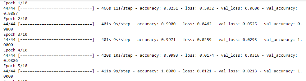
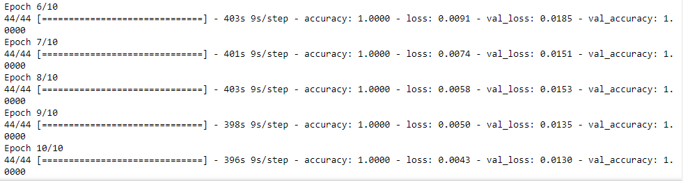
Wow! The model took 4100 seconds, which is almost 1.138 hours to get trained! During the training, both training and validation losses decreased gradually. Although the validation loss suddenly grew a bit twice in the fourth and the eight epochs, it immediately reduced in the very next epochs. Hence, no overfitting was observed.
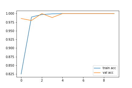
The performance of our model on training and validation datasets can be visualized with the help of accuracy and loss graphs as follows:
# accuracies

plt.plot(history.history['accuracy'], label='train acc')

plt.plot(history.history['val_accuracy'], label='val acc')

plt.legend()

plt.savefig('vgg-acc-rps-1.png')

plt.show()
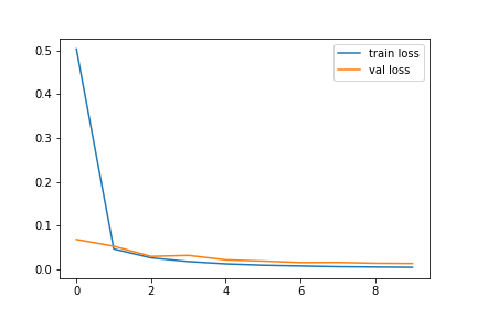
# loss
plt.plot(history.history['loss'], label='train loss')
plt.plot(history.history['val_loss'], label='val loss')
plt.legend()
plt.savefig('vgg-loss-rps-1.png')
plt.show()
Thus, we have successfully trained our VGG-19 model!
Step-4: Model Evaluation
Now, let us evaluate our model by testing it on the test dataset.
model.evaluate(test_x,test_y,batch_size=32)

Awesome! Our model shows a testing accuracy of 99.77% and its testing time is 91 seconds for 437 images.
However, to call our deep learning model good and efficient, it is not only enough to look at its accuracy but it is also equally essential to observe its classification report and confusion matrix. This is another reason behind computing x_test and y_test in step-2.
from sklearn.metrics import accuracy_score,classification_report,confusion_matrix
import numpy as np
#predict
y_pred=model.predict(test_x)
y_pred=np.argmax(y_pred,axis=1)
#get classification report
print(classification_report(y_pred,test_y))
#get confusion matrix
print(confusion_matrix(y_pred,test_y))
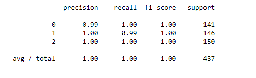
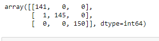
Out of 145 images of rock, all of them have been successfully classified except for 1 image of paper which has been confusedly classified as rock. However, the class of scissors has been perfectly classified. Out of 150 testing images of scissors, all of them have been accurately classified as scissors. But, out of 142 images of papers,141 have been perfectly classified as paper while one image has been wrongly classified as rock.
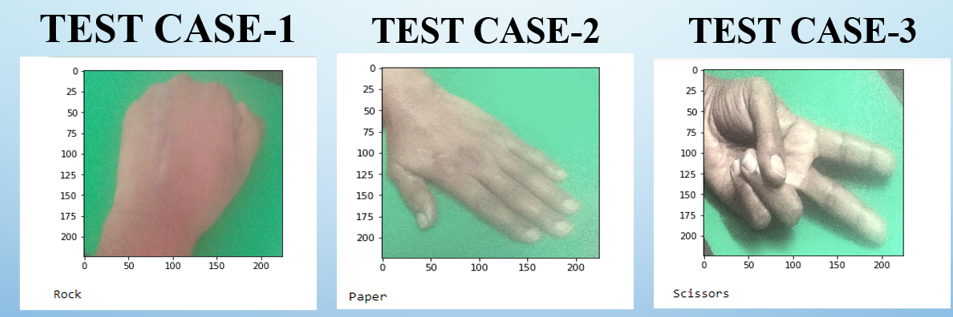
Output screenshot of the results of each of the categories. These are images of my hand gestures.
Therefore, the above results substantiate that the model has successfully classified almost all the images. Therefore, it can undoubtedly be inferred that the model predicts all three classes quite well although not perfectly.
We did it!
Summary
Conclusively, the above steps can be easily followed to build an efficient image classifier for your custom dataset. Thus, in this blog, we have successfully learned how to train a VGG-19 model to classify among rock, paper, and scissors hand gestures. The model can further be trained for more epochs for further better performance. You can extend the take-aways to build one such image classifier for any other custom dataset as well.
You can find the entire code from Github
Hope you enjoyed reading my article.
Thank You
References
2. Evaluating a model in TensorFlow
About Me
I am Nithyashree V, a final year BTech Computer Science and Engineering student. I love learning such cool technologies and putting them into practice, especially observing how they help us solve society’s challenging problems. My areas of interest include Artificial Intelligence, Data Science, and Natural Language Processing.
Here is my LinkedIn profile: My LinkedIn


Hi how are you doing when i train this model using my custom dateset which consist of 30000 train images, 8800 test image and 2000 valid images I get this error : InternalError: Failed copying input tensor from /job:localhost/replica:0/task:0/device:CPU:0 to /job:localhost/replica:0/task:0/device:GPU:0 in order to run _EagerConst: Dst tensor is not initialized. I use GPU NVIDIA RTX 3050 Ti how to fix this error
There is a mistake here. While fitting the model, # fit the model history = model.fit( train_x, train_y, validation_data=(val_x,val_y), epochs=10, callbacks=[early_stop], batch_size=32,shuffle=True) You should have made use of training_set that is augmented data. You are not at all using augemented data. Which you intended by creating training_set. But finally while fitting you are not making use of it. which is a mistake
thanks for this great article, missing parts on how to install tensor flow on MacOSX M1 is: SYSTEM_VERSION_COMPAT=0 pip install tensorflow-macos tensorflow-metal and shortcuts for split dataset images: !!!!Move number of files to dir mv -- *(D.oN[1,456]) ./456 mv -- *(D.oN[1,114]) ./114 hope it save times.