The trinity of errors in applying confidence intervals: An exploration using Statsmodels

Recall from my previous blog post that all financial models are at the mercy of the Trinity of Errors, namely: errors in model specifications, errors in model parameter estimates, and errors resulting from the failure of a model to adapt to structural changes in its environment. Because of this trifecta of errors, we need dynamic models that quantify the uncertainty inherent in our financial estimates and predictions.

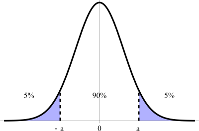
Practitioners in all social sciences, especially financial economics, use confidence intervals to quantify the uncertainty in their estimates and predictions. For example, a 90% confidence interval (CI), as shown in Figure 1, is generally understood to imply that there is a 90% probability that the true value of a parameter of interest is in the interval [-a, a].

In this blog post, we explore the three types of errors in applying CIs that are common in financial research and practice. We develop an ordinary least squares (OLS) linear regression model of equity returns using Statsmodels, a Python statistical package, to illustrate these three error types. We use the diagnostic test results of our regression model to support the reasons why CIs should not be used in financial data analyses.

A significant vote of no confidence in confidence intervals

CI theory was developed around 1937 by Jerzy Neyman, a mathematician and one of the principal architects of modern statistics. Ronald Fisher, the head architect of modern statistics, attacked Neyman’s CI theory by claiming it did not serve the needs of scientists and potentially would lead to mutually contradictory inferences from data. Fisher’s criticisms of CI theory have proved to be justified—but not because Neyman’s CI theory is flawed, as Fisher claimed. Neyman intended his CI theory to be a pre-data theory of statistical inference, developed to inform statistical procedures that have long-run average properties before data are sampled from a population distribution. Neyman made it very clear that his theory was not intended to support inferences after data are sampled in a scientific experiment. CI theory is not a post-data theory of statistical inference despite how it is applied today in research and practice in all social sciences.

Let’s examine the trinity of errors that arises from the common practice of misusing Neyman’s CI theory as a post-data theory—i.e., for making inferences about population parameters based on a specific data sample. The three types of errors using CIs are:

• making probabilistic claims about population parameters
• making probabilistic claims about a specific confidence interval
• making probabilistic claims about sampling distributions

In order to understand this trifecta of errors, we need to understand the fundamental meaning of probability from the perspective of a modern statistician.

Frequently used interpretation of probability

Modern statisticians, such as Fisher and Neyman, claim that probability is a naturally occuring attribute of an event or phenomenon. The probability of an event should be measured empirically by repeating similar experiments ad nauseam—either in reality or hypothetically. For instance, if an experiment is conducted N times and an event E occurs with a frequency M times, the relative frequency M/N approximates the probability of E. As the number of experimental trials N approaches infinity, the probability of E equals M/N.

Statisticians who believe that probability is a natural property of an event and is measured empirically as a long-run relative frequency are called frequentists. Frequentism is the dominant school of statistics of modern times, in both academic research and industrial applications. It is also known as orthodox, classical, modern, or conventional statistics.

Frequentists postulate that the underlying stochastic process that generates data has statistical properties that do not change in the long-run: the probability distribution is time invariant. Even though the parameters of this underlying process may be unknown or unknowable, frequentists believe that these parameters are constant and have “true” values. Population parameters may be estimated from random samples of data. It is the randomness of data that creates uncertainty in the estimates of the true, fixed population parameters. This frequentist philosophy of probability has had a profound impact on the theory and practice of financial economics in general and CIs in particular.

Pricing stocks regressively with Statsmodels

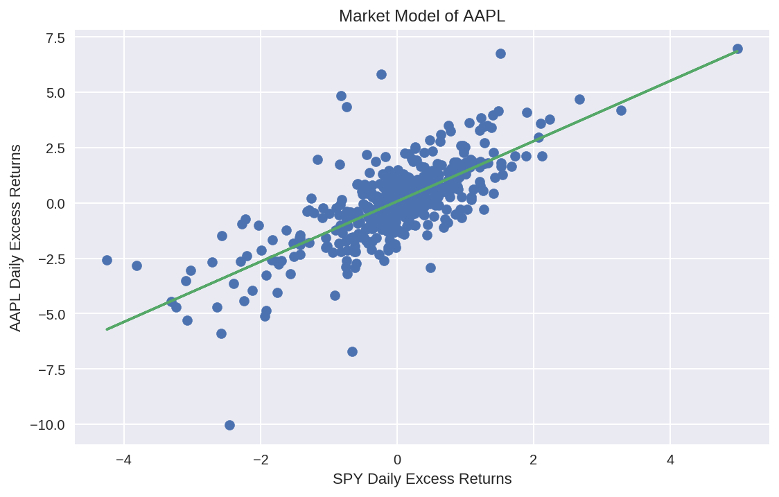
Modern portfolio theory assumes that rational, risk-averse investors demand a risk premium, a return in excess of a risk-free asset such as a treasury bill, for investing in risky assets such as equities. A stock’s single factor market model (MM) is basically a linear regression model of the realized excess returns of a stock (outcome or dependent variable) regressed against the realized excess returns of a single risk factor (predictor or independent variable) such as the overall market as formulated below:

\((R-F) = α + β(M-F) + ϵ\)

Where R is the realized return of a stock, F is the return on a risk-free asset such as a US treasury bill, M is the realized return of a market portfolio such as the S&P 500, α (alpha) is the expected stock-specific return, β (beta) is the level of systematic risk exposure to the market and ε (epsilon) is the unexpected stock-specific return. The beta of a stock gives the average percentage return response to a 1% change in return of the overall market portfolio. For example, if a stock has a beta of 1.4 and the S&P 500 falls by 1%, the stock is expected to fall by -1.4% on average. See Figure 2.

Note that the MM of an asset is different from its Capital Asset Pricing Model (CAPM). The CAPM is the pivotal economic equilibrium model of modern finance that predicts expected returns of an asset based on its 𝛽 or systematic risk exposure to the overall market. Unlike the CAPM, an asset’s MM is a statistical model that has both an idiosyncratic risk term 𝛼 and an error term 𝞮 in its formulation. According to the CAPM, alpha of an asset’s MM has an expected value of zero because market participants are assumed to hold efficient portfolios that diversify the idiosyncratic risks of any specific asset. Market participants are only rewarded for bearing systematic risk since it cannot be diversified away. In keeping with the general assumptions of an OLS regression model, both CAPM and MM assume that the expected value of the residuals 𝞮 to be normally distributed with a zero mean and a constant, finite variance.

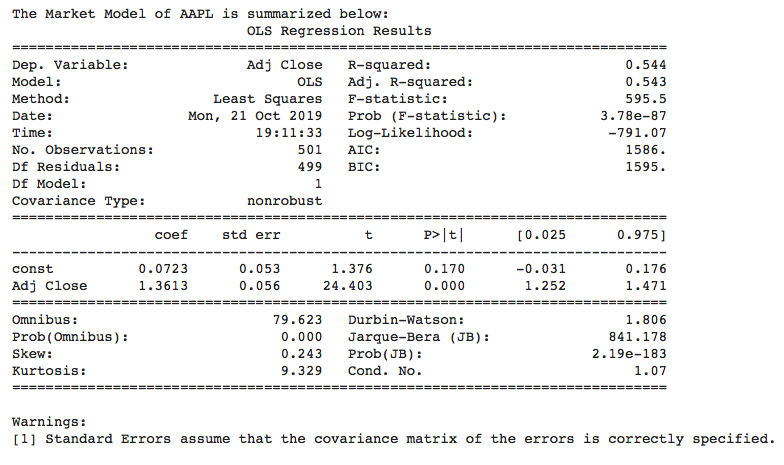
A financial analyst, relying on modern portfolio theory and practice, assumes there is an underlying, time-invariant, stochastic process generating the price data of AAPL which can be modeled as an OLS linear regression MM. This MM will have population parameters, alpha and beta, which have true, fixed values that can be estimated from random samples of AAPL closing price data. Let’s run our Python code (see Jupyter Notebook here) to estimate alpha and beta based on a sample of two years of daily closing prices of AAPL. We can use any holding period return as long as it is used consistently throughout the formula. Using a daily holding period is convenient because it makes price return calculations much easier using Pandas dataframes. After running our Python code, a financial analyst would estimate that alpha is 0.0723% and beta is 1.3613, as shown in the Statsmodels summary output in Figure 3.

Clearly, these point estimates of alpha and beta will vary depending on the sample size, start and end dates used in our random samples, with each estimate reflecting AAPL’s idiosyncratic price fluctuations during that specific time period. Even though the population parameters alpha and beta are unknown, and possibly unknowable, the financial analyst considers them to be true constants of a stochastic process. It is the random sampling of AAPL’s price data that introduces uncertainty in the estimates of constant population parameters. It is the data, and every statistic derived from the data such as CIs, that are treated as random variables. Financial analysts calculate CIs from random samples in order to express the uncertainty around point estimates of constant population parameters.

CIs provide a range of values with a probability value or significance level attached to that range. For instance, in Apple’s MM above, a financial analyst could calculate the 95% confidence interval by calculating the standard error (SE) of alpha and beta. Since the residuals 𝞮 are assumed to be normally distributed with an unknown variance, the t-statistic would to be used in computing CIs. However, because the sample size is greater than 30, the t-distribution converges to the standard normal distribution and the t-statistic values are the same as Z-scores of a standard normal distribution. So, the analyst  would multiply each SE by +/- the Z-score for a 95% CI and then add the result to the point estimate of alpha and beta to obtain its CI. In the Statsmodels results above, the 95% CI for alpha and beta are computed as follows:

α+/- (SE * t-statistic/Z-Score for 95% CI) = 0.0723 % +/- (0.053 % * 1.96) = [-0.032%, 0.176%]

β+/- (SE * t-statistic/Z-Score for 95% CI) = 1.3613 +/- (0.056 * 1.96) = [1.252, 1.471])

The confidence game

What most people think they are getting from a 95% CI is a 95% probability that the true population parameter is within the limits of the specific interval calculated from a specific data sample. For instance, based on the Statsmodels results above, you would think there is a 95% probability that the true value of beta of AAPL is in the range [1.252, 1.471]. Strictly speaking, your interpretation of such a CI would be wrong.

According to Neyman’s CI theory, what a 95% CI actually means is that if we were to draw 100 random samples from the underlying distribution, we would end up with 100 different confidence intervals, and we can be confident that 95 of them will contain the true population parameter within their limits. However, we won’t know which specific 95 CIs of the 100 CIs include the true value of the population parameter and which five CIs do not. We are assured that only the long-run ratio of the CIs that include the population parameter to the ones that do not will approach 95% as we draw random samples ad nauseam.

Winston Churchill could just as well have been talking about CIs instead of Russia’s world war strategy when he said, “It is a riddle, wrapped in a mystery, inside an enigma; but perhaps there is a key.” Indeed, we do present a key in this blog post. Let’s investigate the trifecta of fallacies that arise from misusing CI as a post-data theory in financial data analysis.

Errors in making probabilistic claims about population parameters

Recall that a frequentist statistician considers a population parameter to be a constant with a “true” value. This value may be unknown or even unknowable. But that does not change the fact that its value is fixed. Therefore, a population parameter is either in a CI or it is not. For instance, if you believe the theory that capital markets are highly efficient, you would also believe that the true value of alpha is 0. Now 0 is definitely in the interval [-0.031%, 0.176%] calculated above. Therefore, the probability that alpha is in our CI is 100% and not 95% or any other value.

Because population parameters are believed to be constants by frequentists, there can be absolutely no ambiguity about them: the probability that the true value of a population parameter is within any CI is either 0 or 100%. So, it is erroneous to make probabilistic claims about any population parameter under a frequentist interpretation of probability.

Errors in making probabilistic claims about a specific confidence interval

A more sophisticated interpretation of the above CIs goes as follows: hypothetically speaking, if we were to repeat our linear regression many times, the interval [1.252, 1.471] would contain the true value of beta within its limits about 95% of the time.

Recall that probabilities in the frequentist world apply only to long-run frequencies of repeatable events. By definition, the probability of a unique event, such as a specific CI, is undefined and makes no sense to a frequentist. Therefore, a frequentist cannot assign a 95% probability to either of the specific intervals for alpha and beta that we have calculated above. In other words, we can’t really infer much from a specific CI.

But that is the main objective of our exercise! This limitation of CIs is not very helpful for data scientists who want to make inferences about population parameters from their specific data samples: i.e., they want to make post-data inferences. But, as was mentioned earlier, Neyman intended his CI theory to be used for only pre-data inferences.

Errors in making probabilistic claims about sampling distributions

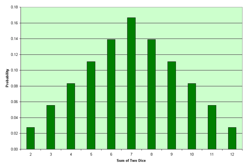
How do financial analysts justify making these probabilistic claims about CIs in research and practice? How do they square the circle? Statisticians can, in theory or in practice, repeatedly sample data from a population distribution. The point estimates of sample means computed from many different random samples create a pattern called the sampling distribution of the sample mean. Sampling distributions enable frequentists to invoke the Central Limit Theorem (CLT) in calculating the uncertainty around sample point estimates of population parameters. In particular, the CLT states that if many samples are drawn randomly from a population with finite variance, the sampling distribution of the sample mean approaches a normal distribution asymptotically. The shape of the underlying population distribution is immaterial and can only affect the speed of this inexorable convergence to normality. Figure 4 demonstrates the power of the CLT by showing how the sampling distribution of the sum of two dice transforms to an approximately normal distribution from the uniform distribution of a single die.

The frequentist definition of probability as a long-run relative frequency of repeatable events resonates with the CLT’s repeated drawing of random samples from a population distribution to generate its sampling distributions. So, statisticians square the circle by invoking the CLT and claiming that their sampling distributions almost surely converge to a normal distribution, regardless of the shape of the underlying population distribution. This also enables them to compute CIs using the Z-scores of the standard normal distribution as shown above.

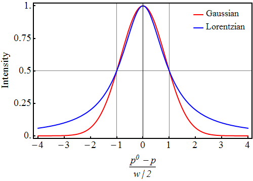
However, you need to read the fine print of the CLT: specifically, you need to note its assumption that the underlying population distribution needs to have a finite mean and variance. While most distributions satisfy these two conditions, there are many that do not. For these types of population distributions, the CLT cannot be invoked to save CIs. For instance, the Cauchy and Pareto distributions are fat-tailed distributions that do not have finite mean and variances. In fact, a Cauchy (or Lorentzian) distribution looks deceptively similar to a normal distribution but has very fat tails because of its infinite variance. See Figure 5.

The diagnostic tests computed by Statsmodels in Figure 3 show us that the equity market has wrecked the key assumptions of our MM. Specifically, the Bera-Jarque and Omnibus normality tests show the probability that the residuals 𝞮 are normally distributed is almost surely zero. This distribution is positively skewed and has very fat tails—a kurtosis that is over three times that of a standard normal distribution.

How about making the sample size even larger? Won’t the distribution of the residuals get more normal with a much larger sample size? Let’s run our MM using 20 years of AAPL’s daily closing prices — 10 times more data than in our previous sample. The results are shown in Figure 6:

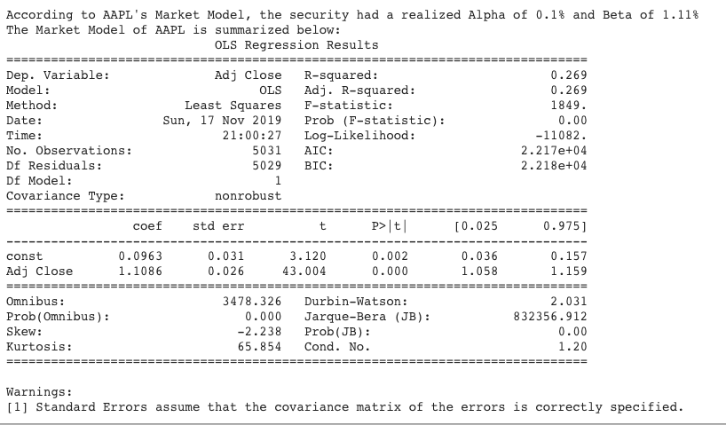
All the diagnostic test results above make it clear that the equity market has savaged the “Nobel-prize” winning CAPM and related MM. Even with a sample size that is 10 times larger than our previous one, the distribution of our model’s residuals is grossly more non-normal than before. It is now very negatively skewed with an absurdly high kurtosis—almost 22 times that of a standard normal distribution. Most notably, the CI of our 20-year beta is [1.058, 1.159], which does not even overlap with the CI of our 2-year beta [1.252,1.471]. In fact, the beta of AAPL seems to be regressing toward 1, the beta value of the S&P 500.

Invoking some version of the CLT and claiming asymptotic normality for the sampling distributions of the residuals or the coefficients of our regression model seem futile, if not invalid. There is a compelling body of economic research claiming that the underlying distributions of all financial asset price returns do not have finite variances. Financial analysts should not be so certain that they can summon the powers of the CLT and assert asymptotic normality in their CI computations. Furthermore, they need to be sure that convergence to asymptotic normality is reasonably fast because, as the eminent economist Maynard Keynes found out the hard way with his equity investments, “Markets can stay irrational longer than you can stay solvent.” For an equity trade, 20 years is an eternity.

Conclusions

Because of the trinity of errors detailed in this blog post, I have no confidence in CIs (or the CAPM or MM for that matter) and do not use it in my financial data analyses. I would not waste a penny trading or investing based on the estimated CIs of alpha and beta of any MM computed by Statsmodels or any other software application.

Neyman’s CI theory is a pre-data theory that is not designed for making post-data inferences. Yet, modern statisticians have concocted a mind-bending, spurious rationale for doing exactly that. Their use of CIs as a post-data theory is epistemologically flawed. It flagrantly violates the philosophical foundation of frequentist probability on which it rests. Of course, this has not stopped data scientists from using CIs blindly or statisticians from teaching it as a mathematically rigorous post-data theory of statistical inference.

You can get away with misusing Neyman’s CI theory if the CLT applies to your data analysis—i.e., the underlying population distribution has a finite mean and variance resulting in asymptotic normality of its sampling distributions. However, it is common knowledge among academics and practitioners that price returns of all financial assets are not normally distributed. It is likely that these fat tails are a consequence of infinite variances of their population distributions. So, the theoretical powers of the CLT cannot be utilized by analysts to rescue CIs from the non-normal, fat-tailed, ugly realities of financial markets. Even if asymptotic normality is theoretically possible in some situations, the desired convergence may not be quick enough for it to be of any practical value for trading and investing. Financial analysts should heed another of Keynes’s warnings when hoping for asymptotic normality of their sampling distributions: “In the long run, we are all dead” (and almost surely broke).

Regardless, financial data analysts using CIs as a post-data theory are making invalid inferences and grossly misestimating the uncertainties in their point estimates. Unorthodox statistical thinking, ground-breaking algorithms, and modern computing technology make the use of CI theory in financial data analysis unnecessary. We will explore such an alternative in the final post of this blog series.

Acknowledgements

I thank Mike Shwe, product manager of TensorFlow Probability at Google Inc., for his feedback on earlier drafts of this blog post.

References

• Probability Theory: The Logic of Science, by E.T. Jaynes, Cambridge University Press, 2003
• The Fallacy Of Placing Confidence In Confidence Intervals, by R.D. Morey, R. Hoekstra et al, Psychonomic Bulletin & Review, 2016
• Quantitative Methods, CFA Program Curriculum, Volume 1, CFA Institute, 2007
• Alternative Investments, CAIA, Level I, John Wiley & Sons, 2015