An Introductory Guide to NLP for Data Scientists with 7 Common Techniques

Modern organizations work with huge amounts of data. That data can come in a variety of different forms including documents, spreadsheets, audio recordings, emails, JSON, and so many, many more. One of the most common ways that such data is recorded is via text. That text is usually quite similar to the natural language that we use from day-to-day.

Natural Language Processing (NLP) is the study of programming computers to process and analyze large amounts of natural textual data. Knowledge of NLP is essential for Data Scientists since text is such an easy to use and common container for storing data.

Faced with the task of performing analysis and building models from textual data, one must know how to perform the basic Data Science tasks. That includes cleaning, formatting, parsing, analyzing, visualizing, and modeling the text data. It’ll all require a few extra steps in addition to the usual way these tasks are done when the data is made up of raw numbers.

This guide will teach you the essentials of NLP when used in Data Science. We’ll go through 7 of the most common techniques that you can use to handle your text data, including code examples with the NLTK and Scikit Learn.

 

(1) Tokenization

Tokenization is the processing of segmenting text into sentences or words. In the process, we throw away punctuation and extra symbols too.

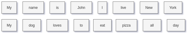
This is not as simple as it looks. For example, the word “New York” in the first example above was separated into two tokens. However, New York is a pronoun and might be quite important in our analysis — we might be better off keeping it in just one token. As such, care needs to be taken during this step.

The benefit of Tokenization is that it gets the text into a format that’s easier to convert to raw numbers, which can actually be used for processing. It’s a natural first step when analyzing text data.

 

(2) Stop Words Removal

A natural next step after Tokenization is Stop Words Removal. Stop Words Removal has a similar goal as Tokenization: get the text data into a format that’s more convenient for processing. In this case, stop words removal removes common language prepositions such as “and”, “the”, “a”, and so on in English. This way, when we analyze our data, we’ll be able to cut through the noise and focus in on the words that have actual real-world meaning.

Stop words removal can be easily done by removing words that are in a pre-defined list. An important thing to note is that there is no universal list of stop words. As such, the list is often created from scratch and tailored to the application being worked on.

 

(3) Stemming

Stemming is another technique for cleaning up text data for processing. Stemming is the process of reducing words into their root form. The purpose of this is to reduce words which are spelled slightly differently due to context but have the same meaning, into the same token for processing. For example, consider using the word “cook” in a sentence. There’s quite a lot of ways we can write the word “cook”, depending on the context:

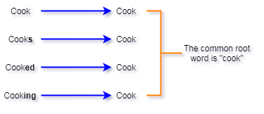
All of these different forms of the word cook have essentially the same definition. So, ideally, when we’re doing our analysis, we’d want them to all be mapped to the same token. In this case, we mapped all of them to the token for the word “cook”. This greatly simplifies our further analysis of the text data.

 

(4) Word Embeddings

Now that our data is cleaned up from those first three methods, we can start converting it into a format that can actually be processed.

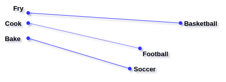
Word embeddings is a way of representing words as numbers, in such a way that words with similar meaning have a similar representation. Modern-day word embeddings represent individual words as real-valued vectors in a predefined vector space.

All word vectors have the same length, just with different values. The distance between two word-vectors is representative of how similar the meaning of the two words is. For example, the vectors of the words “cook” and “bake” will be fairly close, but the vectors of the words “football” and “bake” will be quite different.

A common method for creating word embeddings is called GloVe, which stands for “Global Vectors”. GloVe captures global statistics and local statistics of a text corpus in order to create word vectors.

GloVe uses what’s called a co-occurrence matrix. A co-occurrence matrix represents how often each pair of words occur together in a text corpus. For example, consider how we would create a co-occurrence matrix for the following three sentences:

• I love Data Science.
• I love coding.
• I should learn NLP.

The co-occurrence matrix of this text corpus would look like this:

For a real-world dataset, the matrix would be much, much larger. The good thing is that the word embeddings only have to be computed once for the data and can then be saved to disk.

GloVe is then trained to learn vectors of fixed length for each word, such that the dot product of any two-word vectors equals the logarithm of the words’ probability of co-occurrence, which comes from the co-occurrence matrix. This is represented in the objective function of the paper shown below:

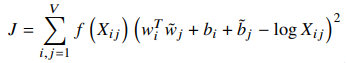
In the equation, X represents the value from the co-occurrence matrix at position (i,j), and the w’s are the word vectors to be learned. Thus, by using this objective function, GloVe is minimizing the difference between the dot product of two-word vectors and the co-occurrence, effectively ensuring that the learned vectors are correlated with the co-occurrence values in the matrix.

Over the past few years, GloVe has proved to be a very robust and versatile word embedding technique, due to its effective encoding of the meanings of the words, and their similarity. For Data Science applications, it’s a battle-tested method for getting words into a format that we can process and analyze.

Here’s a full tutorial about how to use GloVe in Python!

 

(5) Term Frequency-Inverse Document Frequency

Term Frequency-Inverse Document Frequency, more commonly known as TF-IDF is a weighting factor often used in applications such as information retrieval and text mining. TF-IDF uses statistics to measure how important a word is to a particular document.

• TF — Term Frequency:measures how frequently a string occurs in a document. Calculated as the total number of occurrences in the document divided by the total length of the document (for normalization).
• IDF — Inverse Document Frequency:measures the importance of a string within a document. For example, certain strings such as “is”, “of”, and “a”, will appear a lot of times in many documents but don’t really hold much meaning— they’re not adjectives or verbs. IDF, therefore, weights each string according to its importance, calculated as the log() of the total number of documents in the dataset divided by the number of documents that the string occurs in (+1 in the denominator to avoid a division by zero).
• TF-IDF: The final calculation of the TF-IDF is simply the multiplication of the TF and IDF terms: TF * IDF.

The TF-IDF is perfectly balanced, considering both local and global levels of statistics for the target word. Words that occur more frequently in a document are weighted higher, but only if they’re more rare within the whole document.

Due to its robustness, TF-IDF techniques are often used by search engines in scoring and ranking a document’s relevance given a keyword input. In Data Science, we can use it to get an idea of which words, and related information, are the most important in our text data.

 

(6) Topic Modeling

Topic modeling, in the context of NLP, is the process of extracting the main topics from a collection of text data or documents. Essentially, it’s a form of Dimensionality Reduction since we’re reducing a large amount of text data down to a much smaller number of topics. Topic modeling can be useful in a number of Data Science scenarios. To name a few:

• Data analysis of the text — Extracting the underlying trends and main components of the data
• Classifying the text — In a similar way that dimensionality reduction helps with classical Machine Learning problems, topic modeling also helps here since we are compressing the text into the key features, in this case, the topics
• Building recommender systems — topic modeling automatically gives us some basic grouping for the text data. It can even act as an additional feature for building and training the model

Topic modeling is typically done using a technique called Latent Dirichlet Allocation (LDA). With LDA, each text document is modeled as a multinomial distribution of topics, and each topic is modeled as a multinomial distribution of words (individual strings, which we can get from our combination of tokenization, stop words removal, and stemming).

LDA assumes documents are produced from a combination of topics. Those topics then generate words based on their probability distribution.

We start by telling LDA how many topics each document should have, and how many words each topic is made up of. Given a dataset of documents, LDA attempts to determine what combination and distribution of topics can accurately re-create those documents and all the text in them. It can tell which topic(s) works by building the actual documents, where the building is done by sampling words according to the probability distributions of the words, given the selected topic.

Once LDA finds a distribution of topics that can most accurately re-create all of the documents and their contents within the dataset, then those are our final topics with the appropriate distributions.

 

(7) Sentiment Analysis

Sentiment Analysis is an NLP technique that tries to identify and extract the subjective information contained within text data. In a similar way to Topic Modeling, Sentiment Analysis can help transform unstructured text into a basic summary of the information embedded in the data.

Most Sentiment Analysis techniques fall into one of two buckets: rule-based and Machine Learning methods. The rule-based method follows simple steps to achieve their results. After doing some text pre-processing like tokenization, stop words removal, and stemming, a rule-based may, for example, go through the following steps:

1. Define lists of words for the different sentiments. For example, if we are trying to determine if a paragraph is negative or positive, we might define words like badand horrible for the negative sentiment, and great and amazing for the positive sentiment
2. Go through the text and count the number of positive words. Do the same thing for the negative words.
3. If the number of words identified as positive is greater than the number of words identified as negative, then the sentiment of the text is positive— and vice versa for negative

Rule-based methods are great for getting a general idea of how Sentiment Analysis systems work. Modern, state-of-the-art systems, however, will typically use Deep Learning, or at least classical Machine Learning techniques, to automate the process.

With Deep Learning techniques, sentiment analysis is modeled as a classification problem. The text data is encoded into an embedding space (similar to the Word Embeddings describe above) — this is a form of feature extraction. These features are then passed to a classification model where the sentiment of the text is classified.

This learning-based approach is powerful since we can automate it as an optimization problem. The fact that we can continuously feed data to the model to get a continuous improvement out of it is also a huge bonus. More data improves both feature extraction and sentiment classification.

There are a number of great tutorials on how to do Sentiment Analysis with various Machine Learning models. Here are a few great ones:

• With Logistic Regression
• With Random Forest
• With Deep Learning LSTM

Related:

• Automatic Text Summarization in a Nutshell
• Text Encoding: A Review
• Understanding NLP and Topic Modeling Part 1