Estimating the prevalence of rare events — theory and practice
by YI LIU
Importance sampling is used to improve precision in estimating the prevalence of some rare event in a population. In this post, we explain how we use variants of importance sampling to estimate the prevalence of videos that violate community standards on YouTube. We also cover many practical challenges encountered in implementation when the requirement is to produce fresh and regular estimates of prevalence.
Naturally, we get an unbiased estimate of the overall prevalence of violation if we sample the videos uniformly from the population and have them reviewed by human raters to estimate the proportion of violating videos. We also get an unbiased estimate of the violation rate in each policy vertical. But given the low probability of violation and wanting to use our rater capacity wisely, this is not an adequate solution — we typically have too few positive labels in uniform samples to achieve an accurate estimate of the prevalence, especially for those sensitive policy verticals. To obtain a relative error of no more than 20%, we need roughly 100 positive labels, and more often than not, we have zero violation videos in the uniform samples for rarer policies.
Our goal is a better sampling design to improve the precision of the prevalence estimates. This problem can be phrased as an optimization problem — given some fixed review capacity
Of course, any mistakes by the reviewers would propagate to the accuracy of the metrics, and the metrics calculation should take into account human errors. Furthermore, the metrics of interest could involve the prevalence of more than one policy vertical, and the choice of the metrics would affect how we design our sampling and objective function. We will defer rater accuracy and multiple policy verticals to future posts. In this post, we will assume that the raters always give the correct answer, and we only consider the binary label case.
As we note, uniform sampling is unlikely to get enough positive samples to draw inference about the proportion. But importance sampling in statistics is a variance reduction technique to improve the inference of the rate of rare events, and it seems natural to apply it to our prevalence estimation problem. We refer interested readers to [1] (cited here with the author's permission) on the details of importance sampling, and will follow the notation from [1] in what follows.
Suppose there are $N$ videos in the population $V = \{v_1, \ldots, v_N\}$, and $p(v)$ is the probability mass function (PMF) of the video $v$ in $V$, such that $p(v) > 0$, $\sum_i p(v_i) = 1$. The PMF depends on how prevalence is defined. For example, if we care about prevalence in uploaded videos, each video has equal weight $p(v) = \frac{1}{N}$, whereas for prevalence in views, the weight of a video is its share of views during some given period.
As noted, we do not know $f$ precisely but have a good estimate of it in the form of a score $S$. For now, assume that we have a well-calibrated function $g$ such that $$
g(S(v)) = \mathbb{E}_p\left[f(V)|S(V)=S(v)\right]
$$That is, $g$ maps the score to the fraction of videos having that score that are bad. To choose $\tilde{q}$, we first observe that when $f$ is binary, the formula for $\texttt{Var}(\hat{\mu}_q)$ given earlier is minimized by minimizing$$
\sum_{i=1}^N \frac{f(v_i) p(v_i)^2}{q(v_i)}
$$While we cannot minimize this quantity, we can minimize our best guess of it. Thus, optimal q is given by$$
q^* = \arg \min_{q} \sum_{i=1}^N \frac{g(S(v_i))p(v_i)^2}{q(v_i)}
\mbox{ such that } \sum_{i=1}^N q(v_i)=1
$$Applying Lagrange multipliers, this constrained optimization leads to the choice$$
q^*(v) \propto p(v)\sqrt{g(S(v))}
$$Thus, the importance distribution that minimizes the infinite population variance is\begin{align*}
\frac{q(v)}{p(v)} &\propto \sqrt{g(S(v))}\\
&= \sqrt{ \mathbb{E}_p\left[f(V)|S(V)=S(v)\right]}
\end{align*}where $g(v)=\mathbb{E}_p\left[f(V)|S(V)=S(v)\right]$ is the conditional prevalence given the classifier score.
\hat{\mu}_{q, PS} =
\sum_s \tilde{p}(s)
\frac{\sum_{i=1}^N f(v_i) [S(v_i) = s]}{\sum_{i=1}^n [S(v_i) = s]}
$$To see the connection between $\hat{\mu}_{q, PS}$ and $\hat{\mu}_q$, we can rewrite $\hat{\mu}_q$:$$
\hat{\mu}_q = \frac{1}{n}\sum_{i=1}^n f(v_i)\frac{\tilde{p}(S(v_i))}{\tilde{q}(S(v_i))} = \sum_{s}\tilde{p}(s)\frac{\sum_{i=1}^n f(v_i) [S(v_i) = s] }{n\tilde{q}(s)}
$$This shows that $\hat{\mu}_q$ calculates the per stratum prevalence rate using the expected sample size $n\tilde{q}(s)$ in the denominator, whereas $\hat{\mu}_{q,PS}$ divides by the actual number of samples in each stratum.
To see how much of a difference this makes, we can compare the number of unique items in the two sampling schemes. It is clear that there are $n$ unique items in a sampling without replacement. If the unique items in samples with replacement is close to $n$, the influence of individual items on the metric might be small, and we might use sampling without replacement to approximate the procedure of sampling with replacement.
Alternatively, if we allow the sampling size to vary, we could make use of Poisson sampling. Poisson sampling takes a similar idea from the Poisson bootstrap — sampling with replacement is sampling from a multinomial distribution $\texttt{Multinom}(n, (q_1,\ldots, q_N))$. With fixed size $n$, the number of times an individual video $v_i$ occurs in the sample is $\texttt{Binom}(n, q_i)$ marginally, and this can be approximated by the Poisson distribution $\texttt{Pois}(n q_i)$ when $nq_i$ is not large.
First, we cannot assume the metric we calculate is a good approximation of the "true metric". If missingness of the verdict is correlated with the label, ignoring missing items might bias the metric. For example, if positive items take longer time to verify because of additional steps, then ignoring those items might underestimate the prevalence metric. We cannot correct such biases in our estimators, and to limit the impact of the missing verdicts, we should wait to compute the metrics until the missing verdict rate is small.
Second, even if the missing verdict rate is small, we might still need to modify our estimators to adjust for it. For the importance sampling estimator $\hat{\mu}_q$, we divide the weighted sum by the number of samples $n$, and with missing verdicts, it seems natural to calculate the metrics using only reviewed items and divide the weighted sum by the number of reviewed samples $n^*$. However, if the missing verdict rate depends on the classifier score, then we may have $$
\mathbb{E}_q \left[\frac{p(V)}{q(V)} |V \text{ is reviewed} \right] \neq 1
$$Because our derivation of importance sampling required that $\mathbb{E}_q \left[\frac{p(V)}{q(V)} \right] = 1$, using $n^*$ as the denominator may be biased. But this can happen easily in practice. For example, if we want to remove bad content from the platform as soon as possible, we may prioritize reviewing the content with the highest classifier scores, and the ones missing review are more likely to be those videos with low classifier scores.
Suppose we accept the missing at random (MAR) assumption, that the probability the video is missing a verdict is independent of its label given the classifier score. In this case, we can remove bias by using the post-stratification estimator $\mu_{q, PS}$. Under the MAR assumption, both the strata weights in the target distribution $p$ and the conditional prevalence rate is unbiased. Even if this MAR assumption is not true, post-stratification seems a more robust estimator than the importance sampling estimator.
First, if the classifier prediction is a bona fide probability of the video being bad, we can use the score directly. This is straightforward and easy to implement. But we find that the predicted score is often calibrated to the training data. When training a classifier with few positives in the population, one common strategy is to over sample items with positive labels, and/or down sample items with negative labels. The ratio between positive and negative samples in the training data directly affects the probability score of the classifier, so the classifier score usually is not calibrated to the probability.
In this situation, we may use historical data to estimate the conditional prevalence rate. Say we observe $(S(v_i), f(v_i))$ pair from past samples, and we would like to calculate $g(s) = \mathbb{E}_p\left[f(V)|S(V)= s \right]$ from the observations. With finite observations on a continuous classifier score $S(v_i)$, the sample conditional prevalence in the stratum would make for a volatile estimation. There are two ideas to improve the estimates:
Whether or not we borrow strength from other scores also impacts the estimation. In our case when the population prevalence rate is low, it is quite common to have few positive items in historical samples for when the classifier score is low. The regression method extrapolates the prevalence of high score regions and extends the estimate to low score regions. On the other hand, the bucketing method might put 0 as the prevalence rate if no positive items occur in the bucket, and the importance sampling distribution using this prevalence rate would not sample any new items from the region (we could adjust the bucket boundary to avoid that).
When we fit the historical data, it is important to be aware of the following caveats:
All methods discussed in this section rely on past data (either from training data or historical samples). However, the distribution of bad videos might not remain constant over time due to the adversarial nature of the problem. For example, if the video violation is correlated with classifier score, bad actors might upload more videos that are harder to detect by the classifiers, resulting in a shifting of conditional prevalence over time. To mitigate this issue, we may limit to only using recent data, or adding a time decay function to down-weight items further in the past.
More generally, we can apply defensive importance sampling [8] in which the importance sampling distribution is a mixture of our target distribution $p$ and the estimated importance distribution $\hat{q}$ to deal with shifts in either conditional prevalence or the region where the prevalence is most uncertain:$$
{\hat{q}_{\lambda}(v)} = \lambda p(v)+ (1 - \lambda){\hat{q}(v)}
$$With the mixture distribution, we can guaranteed that inverse sampling ratio $$
\frac{p(v)}{\hat{q}_{\lambda}(v)} \leq 1 / \lambda
$$ is bounded above, and we can allocate enough samples even when $\hat{q}$ is very small in the regions with few positives (or few negatives using optimal weight from post-stratification). The choice of $\lambda$ would be a small value between 0.1 and 0.5 as estimated from the data (details in [8]).
However, in the case of binomial proportions far from $\frac{1}{2}$, estimates of $\hat{\mu}_q$ and $\hat{\mu}_{q, PS}$ on finite samples converge poorly to the true uncertainty. As a result, confidence intervals from the z-distribution have poor coverage (see [2]).
To demonstrate this issue, consider the following toy example with categorical scores:
The sampling proportions are chosen to be optimal for post-stratification. The following chart shows the point estimate and z-confidence interval of this toy example with 400 Monte Carlo simulations. From the chart, as the sample size increases from 1,000 to 100,000, the length of the confidence interval is more consistent, and the mis-coverage case is more uniformly distributed on both sides.
The situation is slightly better when we have a larger sample, but even with 10,000 samples (expected 6.7 positive in the low risk bucket), having 5 or fewer positive samples (about 1/3 of the chance) would result in the standard error being at least 9% smaller than the theoretical standard deviation.
Under-estimation of standard error essentially happens when we do not have enough positives in certain regions. But here is the thing — importance sampling makes the problem worse by down-sampling such regions, resulting in even more sparse positive items!
Luckily, the binomial proportion estimation literature contains several methods other than the normal approximation interval (the Wald interval), and [3] suggests using either the Jeffreys interval, the Agresti-Coull interval, or the Wilson score interval to estimate the proportion. Jeffreys interval is a Bayesian posterior interval with prior $\texttt{Beta}(\frac{1}{2}, \frac{1}{2})$. The Agresti-Coull interval adds pseudo counts 2 to success and failures before using the normal approximation, and the center of the Wilson score interval may also be interpreted as adding pseudo counts. Thus all these methods are connected to adding pseudo counts and shrinking the point estimate towards $\frac{1}{2}$.
When we use post-stratification in our importance sampling, we could apply a similar idea to estimate the standard error (or posterior interval for Bayesian methods) in each stratum before combining them into an overall CI. But none of these methods yields a satisfactory result in our case because the positive events are rare, and shrinking the prevalence estimate to $\frac{1}{2}$ will overestimate the true prevalence. An alternative is to the Stratified Wilson Interval estimate [3] such the pseudo counts added to each stratum depend on the overall interval width.
Of course, which CI method works best for the problem depends on many factors and no method is universally better than others. In our problem, the stratified Wilson interval works well for our video sampling problem.
To demonstrate the performance of different CI methods, we created a synthetic data with 5 strata that is similar to our video sampling problem. The following chart shows the coverage of 95% CI of different methods for each method under different sample sizes using 4000 simulations.
There is an additional benefit of having coarse strata — it makes it harder for videos to move into different buckets when we retrain a new version of the classifier. This makes aggregating the metrics over multiple periods more robust, as we may sample items on different days with different versions of the classifier.
Cochran recommends no more than 6 or 7 strata [4] while others [5] suggest little to gained from going beyond 5 to 10 strata. Once you fix strata size, you might consider using the Danlenius-Hodges method [6] to select strata boundary.
[2] Lawrence Brown, Tony Cai, Anirban DasGupta (2001). Interval Estimation for a Binomial Proportion. Statistical Science. 16 (2): 101–133.
[3] Xin Yan, Xiao Gang Su. Stratified Wilson and Newcombe Confidence Intervals for Multiple Binomial Proportions. Statistics in Biopharmaceutical Research, 2010.
[4] William Cochran (1977). Sampling Techniques pp 132-134.
[5] Ray Chambers, Robert Clark (2012). An Introduction to Model-Based Survey Sampling with Applications.
[6] Tore Dalenius, Joseph Hodges (1959). Minimum Variance Stratification. Journal of the American Statistical Association, 54, 88-101.
[7] Neyman, J. (1934). “On the Two Different Aspects of the Representative Method: The Method of Stratified Sampling and the Method of Purposive Selection”, Journal of the Royal Statistical Society, Vol. 97, 558-606.
[8] Tim Hesterberg (1995). Weighted Average Importance Sampling and Defensive Mixture Distributions. Technometrics, 37(2): 185 - 192.
Importance sampling is used to improve precision in estimating the prevalence of some rare event in a population. In this post, we explain how we use variants of importance sampling to estimate the prevalence of videos that violate community standards on YouTube. We also cover many practical challenges encountered in implementation when the requirement is to produce fresh and regular estimates of prevalence.
Background
Every day, millions of videos are uploaded to YouTube. While most of these videos are safe for everyone to enjoy, some videos violate the community guidelines of YouTube and should be removed from the platform. There is a wide range of policy violations, from spammy videos, to videos containing nudity, to those with harassing language. We want to estimate the prevalence of violation of each individual policy category (we call them policy verticals) by sampling the videos and manually reviewing those sampled videos.Naturally, we get an unbiased estimate of the overall prevalence of violation if we sample the videos uniformly from the population and have them reviewed by human raters to estimate the proportion of violating videos. We also get an unbiased estimate of the violation rate in each policy vertical. But given the low probability of violation and wanting to use our rater capacity wisely, this is not an adequate solution — we typically have too few positive labels in uniform samples to achieve an accurate estimate of the prevalence, especially for those sensitive policy verticals. To obtain a relative error of no more than 20%, we need roughly 100 positive labels, and more often than not, we have zero violation videos in the uniform samples for rarer policies.
Our goal is a better sampling design to improve the precision of the prevalence estimates. This problem can be phrased as an optimization problem — given some fixed review capacity
- how should we sample videos?
- how do we calculate the prevalence rate from these samples (with confidence intervals)?
Of course, any mistakes by the reviewers would propagate to the accuracy of the metrics, and the metrics calculation should take into account human errors. Furthermore, the metrics of interest could involve the prevalence of more than one policy vertical, and the choice of the metrics would affect how we design our sampling and objective function. We will defer rater accuracy and multiple policy verticals to future posts. In this post, we will assume that the raters always give the correct answer, and we only consider the binary label case.
Importance sampling
In the binary label problem, a video will be either labeled good or bad. Usually, bad videos only make up a tiny proportion of the population, so the two labels are highly imbalanced. Our goal here is to have an accurate and precise estimate of the proportion of bad videos in the population by sampling.As we note, uniform sampling is unlikely to get enough positive samples to draw inference about the proportion. But importance sampling in statistics is a variance reduction technique to improve the inference of the rate of rare events, and it seems natural to apply it to our prevalence estimation problem. We refer interested readers to [1] (cited here with the author's permission) on the details of importance sampling, and will follow the notation from [1] in what follows.
Suppose there are $N$ videos in the population $V = \{v_1, \ldots, v_N\}$, and $p(v)$ is the probability mass function (PMF) of the video $v$ in $V$, such that $p(v) > 0$, $\sum_i p(v_i) = 1$. The PMF depends on how prevalence is defined. For example, if we care about prevalence in uploaded videos, each video has equal weight $p(v) = \frac{1}{N}$, whereas for prevalence in views, the weight of a video is its share of views during some given period.
Furthermore, let $B$ be the set of all bad videos. Define $f(v) = [v \in B]$ where $[\cdot]$ maps the boolean value of the expression contained within to $0$ or $1$. Then the proportion of bad videos is $$
\mu = P_p(B) = \sum_{i = 1} ^N f(v_i) p(v_i) = \mathbb{E}_{p}[f(V)]
$$If $q$ is another PMF defined on the videos such that $q(v_i) > 0$, $\sum_{i=1} ^N q(v_i) = 1$, then we could also write the proportion as$$
\mu = \sum_{i=1}^N f(v_i) q(v_i) \cdot \frac{p(v_i)}{q(v_i)} = \mathbb{E}_q\left[ f(V) \frac{p(V)}{q(V)}\right]$$
Instead of uniformly sampling from the target distribution $p$, importance sampling allows us to sample $n$ items $v_1, \ldots, v_n$ from the population with replacement (more on this later) using the importance distribution $q$, and to correct the sampling bias by inverse-weighting the sampling ratio $q / p$ in the estimator:$$
\hat{\mu}_q =\frac{1}{n} \sum_{i = 1} ^ n f(v_i) \cdot \frac{p(v_i)}{q(v_i)}
$$It is easy to show that the importance sampling estimator is unbiased for $\mu$. The variance of $\hat{\mu}_q$ is\begin{align*}
\texttt{Var}(\hat{\mu}_q) &=
\frac{1}{N}\sum_{i=1}^N \frac{\left(f(v_i)p(v_i) \right)^2}{q(v_i)} -\mu^2 \\
&= \frac{1}{N}\sum_{i=1}^N \frac{\left(f(v_i)p(v_i) - \mu q(v_i)\right)^2}{q(v_i)}
\end{align*}The variance of our estimator depends on the proposed importance distribution $q$, and with appropriate choice of $q$, we can have a better estimator than by uniform sampling.
From the equation above, the variance is minimized when $$q \propto f \cdot p$$that is, when $q$ is proportional to the target distribution $p$ on the set $B$, and 0 outside the set $B$. Unfortunately, this perfect importance distribution requires us to know $f$. If we could separate bad videos from good videos perfectly, we could simply calculate the metrics directly without sampling. But in a world without perfect knowledge of $f$, the heuristic still holds — if we have an approximate rule to separate bad videos from the good ones, we could use it to design our importance distribution $q$. A machine learning classifier serves this task perfectly.
Formally, let $S(v)$ be the real-valued classifier score for video $v$ (if the score is categorical, we assume it has some number of distinct levels). The classifier score $S(v)$ contains whatever information we have about the chances that the video is bad — if two videos have the same score $S(v_1) = S(v_2)$, then the ratio in the importance distribution $q$ should be the same as the ratio in the target distribution $p$, i.e. $$
S(v_1) = S(v_2) \implies \frac{q(v_1)}{p(v_1)} = \frac{q(v_2)}{p(v_2)}$$The ratio between the importance distribution and target distribution is thus a function of $S(v)$:$$
\frac{q(v)}{p(v)} = \frac{\tilde{q}(S(v))}{\tilde{p}(S(v))}
$$where $\tilde{p}$ and $\tilde{q}$ are PMFs of $S(v)$ under the target distribution and importance distribution respectively.
As noted, we do not know $f$ precisely but have a good estimate of it in the form of a score $S$. For now, assume that we have a well-calibrated function $g$ such that $$
g(S(v)) = \mathbb{E}_p\left[f(V)|S(V)=S(v)\right]
$$That is, $g$ maps the score to the fraction of videos having that score that are bad. To choose $\tilde{q}$, we first observe that when $f$ is binary, the formula for $\texttt{Var}(\hat{\mu}_q)$ given earlier is minimized by minimizing$$
\sum_{i=1}^N \frac{f(v_i) p(v_i)^2}{q(v_i)}
$$While we cannot minimize this quantity, we can minimize our best guess of it. Thus, optimal q is given by$$
q^* = \arg \min_{q} \sum_{i=1}^N \frac{g(S(v_i))p(v_i)^2}{q(v_i)}
\mbox{ such that } \sum_{i=1}^N q(v_i)=1
$$Applying Lagrange multipliers, this constrained optimization leads to the choice$$
q^*(v) \propto p(v)\sqrt{g(S(v))}
$$Thus, the importance distribution that minimizes the infinite population variance is\begin{align*}
\frac{q(v)}{p(v)} &\propto \sqrt{g(S(v))}\\
&= \sqrt{ \mathbb{E}_p\left[f(V)|S(V)=S(v)\right]}
\end{align*}where $g(v)=\mathbb{E}_p\left[f(V)|S(V)=S(v)\right]$ is the conditional prevalence given the classifier score.
Post-stratification
When the probability of sampling video $v$ depends only on its score $S(v)$, importance sampling is the same as random sampling within the same score category. We can leverage the score information and use post-stratification to reduce the strata variability introduced by sampling:$$\hat{\mu}_{q, PS} =
\sum_s \tilde{p}(s)
\frac{\sum_{i=1}^N f(v_i) [S(v_i) = s]}{\sum_{i=1}^n [S(v_i) = s]}
$$To see the connection between $\hat{\mu}_{q, PS}$ and $\hat{\mu}_q$, we can rewrite $\hat{\mu}_q$:$$
\hat{\mu}_q = \frac{1}{n}\sum_{i=1}^n f(v_i)\frac{\tilde{p}(S(v_i))}{\tilde{q}(S(v_i))} = \sum_{s}\tilde{p}(s)\frac{\sum_{i=1}^n f(v_i) [S(v_i) = s] }{n\tilde{q}(s)}
$$This shows that $\hat{\mu}_q$ calculates the per stratum prevalence rate using the expected sample size $n\tilde{q}(s)$ in the denominator, whereas $\hat{\mu}_{q,PS}$ divides by the actual number of samples in each stratum.
With the estimator $\hat{\mu}_{q, PS}$, the optimal sampling weight is proportional to the stratum standard error (see [7]):\begin{align*}
\frac{q(v)}{p(v)}
&\propto
\sqrt{g(S(v)) \left(1 - g(S(v)) \right) } \\
&=
\sqrt{ \mathbb{E}_p\left[f(V)|S(V)=S(v)\right] \left( 1 - \mathbb{E}_p\left[f(V)|S(V)=S(v)\right]\right) }
\end{align*}The biggest difference between post-stratification and importance sampling is that the optimal sampling weight for post-stratification peaks at the conditional prevalence rate of $\frac{1}{2}$, while the optimal weight for importance sampling is monotone increasing as conditional prevalence rate increases. In our case when the events are rare and the probability of high conditional prevalence rate is small under the target distribution, the difference between the methods is minor. But in other applications, using post-stratification might further reduce the variance to a significant degree.
We discuss other practical benefits of post-stratification estimator $\mu_{q,PS}$ in the next section.
Complications of implementation
So far, we have seen how importance sampling and post-stratification can provide an unbiased, more precise estimate of prevalence of bad videos. In reality, there are many factors that might affect the unbiasedness and precision of the estimator. In this section, we focus on the practical issues of sampling and estimation, especially how different conditions might affect our estimator. We also discuss how to choose $q$ with respect to the conditional prevalence rate $g(S(v))=\mathbb{E}_p\left[f(V)|S(V)=S(v)\right]$.Sampling algorithm
If the sample size $n$ is fixed, sampling algorithms could be classified as sampling with replacement or sampling without replacement. The difference between the two is whether the same item can appear in the sample multiple times. Our estimators $\mu_{q}$ and $\mu_{q, PS}$ rely on the assumption of sampling with replacement. The measurement may be biased if our samples are generated from a procedure that samples without replacement, such as reservoir sampling, especially if some items have disproportionate weight, i.e., $q(v_i) \cdot n$ is large. For videos and other web content, it is common for the most popular items to account for a significant fraction of views.To see how much of a difference this makes, we can compare the number of unique items in the two sampling schemes. It is clear that there are $n$ unique items in a sampling without replacement. If the unique items in samples with replacement is close to $n$, the influence of individual items on the metric might be small, and we might use sampling without replacement to approximate the procedure of sampling with replacement.
The number of unique items in sampling with replacement is\begin{align*}
\sum_{i=1}^N\left[1 - (1 - q(v_i))^n\right]
&\approx
\sum_{i=1}^N\left[ n q(v_i) - \frac{n^2}{2} q(v_i)^2 \right] \\
&= n - \frac{n^2}{2} \sum_{i=1}^N q(v_i)^2
\end{align*}So the expected number of unique items is controlled by $n ^ 2 \sum_{i=1}^N q(v_i)^2$, and we should be able to use sampling without replacement if $q(v_i)^2$ is small.
With this insight, we could artificially split all videos to $k$ independent copies $(v_i, q_i) \rightarrow (v_i, q_i/k), \ldots, (v_i, q_i/k)$, so each item might appear in the sample at most $k$ times. The sum of weights squared after splitting is $\sum_{i=1}^N q_i^2 / k$, and thus mitigates the problem of skewness in the weights.
Alternatively, if we allow the sampling size to vary, we could make use of Poisson sampling. Poisson sampling takes a similar idea from the Poisson bootstrap — sampling with replacement is sampling from a multinomial distribution $\texttt{Multinom}(n, (q_1,\ldots, q_N))$. With fixed size $n$, the number of times an individual video $v_i$ occurs in the sample is $\texttt{Binom}(n, q_i)$ marginally, and this can be approximated by the Poisson distribution $\texttt{Pois}(n q_i)$ when $nq_i$ is not large.
Missing reviews
One challenge we have with human eval data is that we don't have individual verdict $f(v_i)$ immediately after sampling, and it takes time before we can use it to calculate the metric. Quite often, when we calculate the prevalence metrics, the number of samples with a verdict $n^*$ is smaller than the total sample size. The missing verdicts create two problems.First, we cannot assume the metric we calculate is a good approximation of the "true metric". If missingness of the verdict is correlated with the label, ignoring missing items might bias the metric. For example, if positive items take longer time to verify because of additional steps, then ignoring those items might underestimate the prevalence metric. We cannot correct such biases in our estimators, and to limit the impact of the missing verdicts, we should wait to compute the metrics until the missing verdict rate is small.
Second, even if the missing verdict rate is small, we might still need to modify our estimators to adjust for it. For the importance sampling estimator $\hat{\mu}_q$, we divide the weighted sum by the number of samples $n$, and with missing verdicts, it seems natural to calculate the metrics using only reviewed items and divide the weighted sum by the number of reviewed samples $n^*$. However, if the missing verdict rate depends on the classifier score, then we may have $$
\mathbb{E}_q \left[\frac{p(V)}{q(V)} |V \text{ is reviewed} \right] \neq 1
$$Because our derivation of importance sampling required that $\mathbb{E}_q \left[\frac{p(V)}{q(V)} \right] = 1$, using $n^*$ as the denominator may be biased. But this can happen easily in practice. For example, if we want to remove bad content from the platform as soon as possible, we may prioritize reviewing the content with the highest classifier scores, and the ones missing review are more likely to be those videos with low classifier scores.
Suppose we accept the missing at random (MAR) assumption, that the probability the video is missing a verdict is independent of its label given the classifier score. In this case, we can remove bias by using the post-stratification estimator $\mu_{q, PS}$. Under the MAR assumption, both the strata weights in the target distribution $p$ and the conditional prevalence rate is unbiased. Even if this MAR assumption is not true, post-stratification seems a more robust estimator than the importance sampling estimator.
Choosing the importance distribution
We have that seen the optimal importance distribution $q*$ depends on the conditional prevalence rate and the target distribution (it also depends whether we use post-stratification or not), but the conditional prevalence rate is unknown and needs to be estimated. There are many strategies we can use to estimate this quantity, and we will discuss each option in detail.First, if the classifier prediction is a bona fide probability of the video being bad, we can use the score directly. This is straightforward and easy to implement. But we find that the predicted score is often calibrated to the training data. When training a classifier with few positives in the population, one common strategy is to over sample items with positive labels, and/or down sample items with negative labels. The ratio between positive and negative samples in the training data directly affects the probability score of the classifier, so the classifier score usually is not calibrated to the probability.
In this situation, we may use historical data to estimate the conditional prevalence rate. Say we observe $(S(v_i), f(v_i))$ pair from past samples, and we would like to calculate $g(s) = \mathbb{E}_p\left[f(V)|S(V)= s \right]$ from the observations. With finite observations on a continuous classifier score $S(v_i)$, the sample conditional prevalence in the stratum would make for a volatile estimation. There are two ideas to improve the estimates:
- We might smooth the estimation by fitting a regression on the given data. For example, we could fit a logistic regression on a smooth transform of $(S(v_i)$ (e.g. polynomial or spline) to estimate the conditional prevalence. This reduces the number of parameters to estimate.
- We may also reduce the number of parameters we need to estimate, by bucketing the $S(v_i)$ into a few discrete buckets and estimating the prevalence rate within each bucket. By reducing the parameters we want to estimate, the sparse observations become dense, and we will have a better estimation of each classifier bucket.
Whether or not we borrow strength from other scores also impacts the estimation. In our case when the population prevalence rate is low, it is quite common to have few positive items in historical samples for when the classifier score is low. The regression method extrapolates the prevalence of high score regions and extends the estimate to low score regions. On the other hand, the bucketing method might put 0 as the prevalence rate if no positive items occur in the bucket, and the importance sampling distribution using this prevalence rate would not sample any new items from the region (we could adjust the bucket boundary to avoid that).
When we fit the historical data, it is important to be aware of the following caveats:
- The estimates depend on the distribution of historical samples, which need not be identical to the target distribution. If we use importance sampling on historical samples, we would inversely weigh each observation in the sample and fit a weighted regression or weighted average to form a better estimate.
- In regression, the scale of the classifier score $S(v_i)$ matters. Because binary classifiers often use softmax to normalize the predicted score, it makes sense to reverse the predicted score $S(v_i)$ with the logit function and fit the regression on the real line.
More generally, we can apply defensive importance sampling [8] in which the importance sampling distribution is a mixture of our target distribution $p$ and the estimated importance distribution $\hat{q}$ to deal with shifts in either conditional prevalence or the region where the prevalence is most uncertain:$$
{\hat{q}_{\lambda}(v)} = \lambda p(v)+ (1 - \lambda){\hat{q}(v)}
$$With the mixture distribution, we can guaranteed that inverse sampling ratio $$
\frac{p(v)}{\hat{q}_{\lambda}(v)} \leq 1 / \lambda
$$ is bounded above, and we can allocate enough samples even when $\hat{q}$ is very small in the regions with few positives (or few negatives using optimal weight from post-stratification). The choice of $\lambda$ would be a small value between 0.1 and 0.5 as estimated from the data (details in [8]).
Confidence Intervals
Besides the point estimate of the prevalence metric, we are also interested in constructing a confidence interval to indicate the accuracy of the estimate. Typically, we have the variance formula for $\hat{\mu}_q$ or $\hat{\mu}_{q, PS}$, and we could use a z-score to calculate the confidence interval of the metric.However, in the case of binomial proportions far from $\frac{1}{2}$, estimates of $\hat{\mu}_q$ and $\hat{\mu}_{q, PS}$ on finite samples converge poorly to the true uncertainty. As a result, confidence intervals from the z-distribution have poor coverage (see [2]).
To demonstrate this issue, consider the following toy example with categorical scores:
The sampling proportions are chosen to be optimal for post-stratification. The following chart shows the point estimate and z-confidence interval of this toy example with 400 Monte Carlo simulations. From the chart, as the sample size increases from 1,000 to 100,000, the length of the confidence interval is more consistent, and the mis-coverage case is more uniformly distributed on both sides.
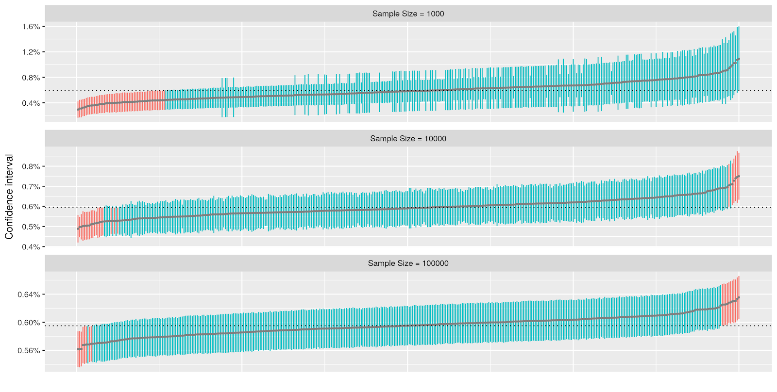 |
| Confidence intervals ordered by the point estimate. Uncovered intervals are red. |
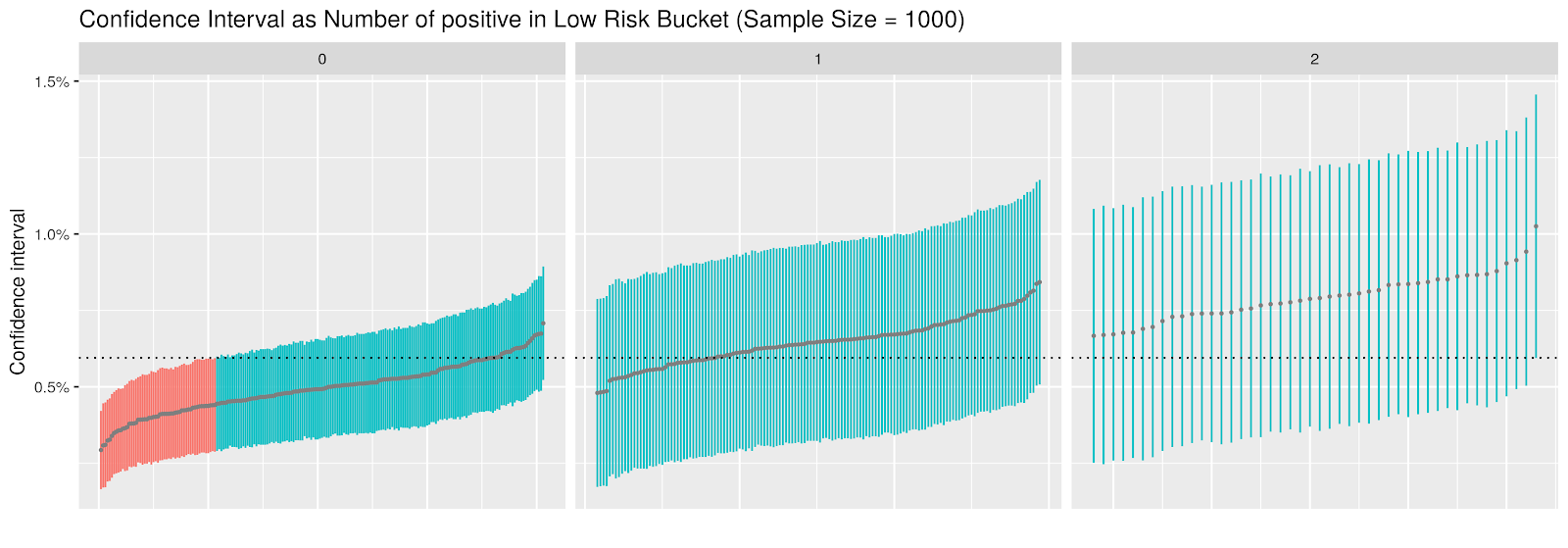
If we zoom in to the case with 1,000 samples, we see that the CI width is highly correlated with the number of positive items in the low risk bucket. When there are no positives in that bucket, the sample standard error is on average 40% smaller than the one using theoretical standard deviation, resulting in poor coverage.
Under-estimation of standard error essentially happens when we do not have enough positives in certain regions. But here is the thing — importance sampling makes the problem worse by down-sampling such regions, resulting in even more sparse positive items!
Luckily, the binomial proportion estimation literature contains several methods other than the normal approximation interval (the Wald interval), and [3] suggests using either the Jeffreys interval, the Agresti-Coull interval, or the Wilson score interval to estimate the proportion. Jeffreys interval is a Bayesian posterior interval with prior $\texttt{Beta}(\frac{1}{2}, \frac{1}{2})$. The Agresti-Coull interval adds pseudo counts 2 to success and failures before using the normal approximation, and the center of the Wilson score interval may also be interpreted as adding pseudo counts. Thus all these methods are connected to adding pseudo counts and shrinking the point estimate towards $\frac{1}{2}$.
When we use post-stratification in our importance sampling, we could apply a similar idea to estimate the standard error (or posterior interval for Bayesian methods) in each stratum before combining them into an overall CI. But none of these methods yields a satisfactory result in our case because the positive events are rare, and shrinking the prevalence estimate to $\frac{1}{2}$ will overestimate the true prevalence. An alternative is to the Stratified Wilson Interval estimate [3] such the pseudo counts added to each stratum depend on the overall interval width.
Of course, which CI method works best for the problem depends on many factors and no method is universally better than others. In our problem, the stratified Wilson interval works well for our video sampling problem.
To demonstrate the performance of different CI methods, we created a synthetic data with 5 strata that is similar to our video sampling problem. The following chart shows the coverage of 95% CI of different methods for each method under different sample sizes using 4000 simulations.
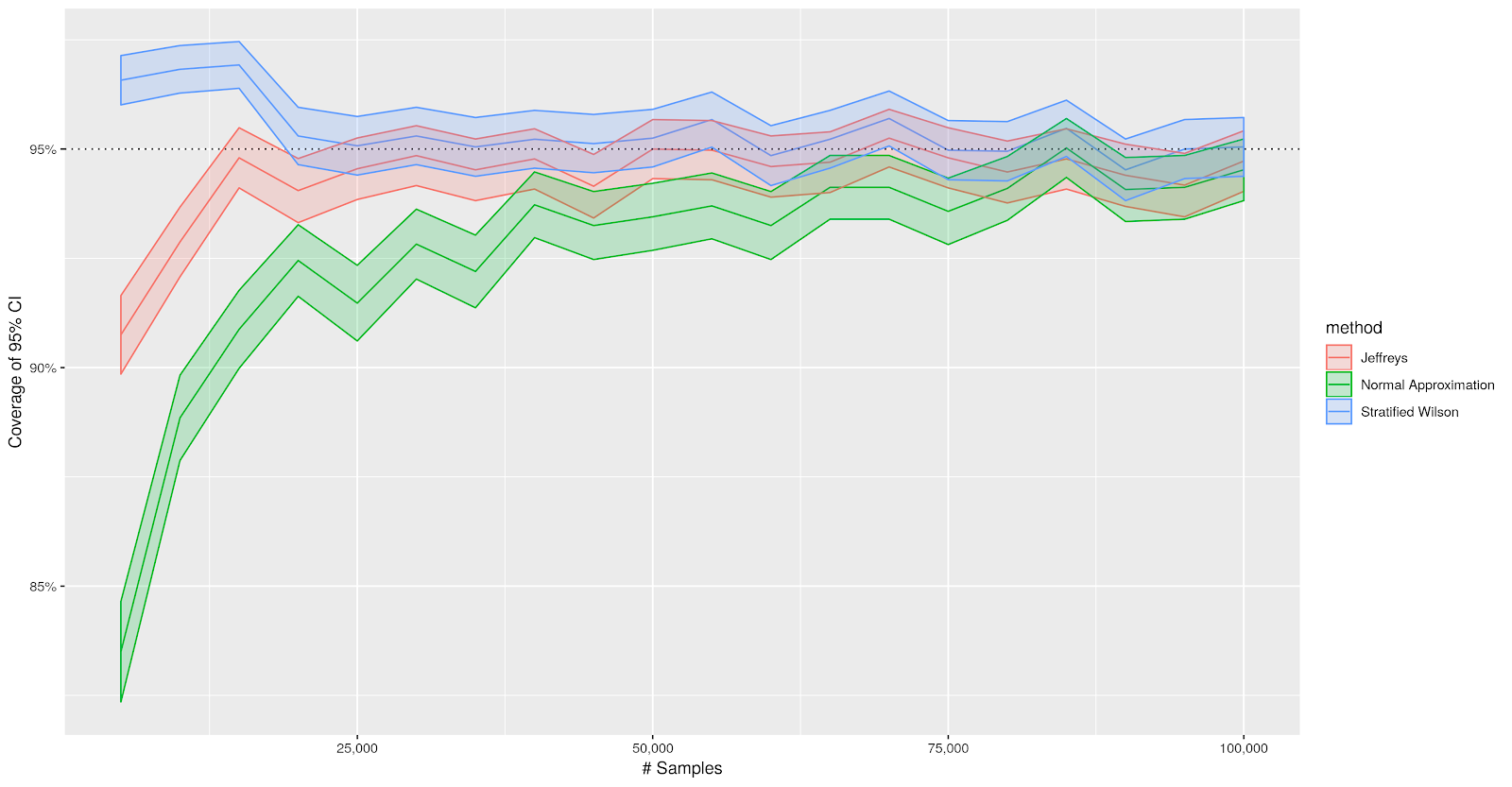 |
| Coverage of 95% CIs with 95% confidence bands. |
We see that confidence intervals using the normal approximation perform poorly until we have about 100,000 samples. Jeffreys CI under-covers when the number of samples is small, while the stratified Wilson CI is a little more conservative, having coverage greater than nominal.
If we drill down into the cases when the CIs do not cover the true prevalence rate, it is clear that Jeffreys CI tends to overestimate the CI (the lower end of the CI is above the ground truth). This happens because the prior shrinks the estimate towards $\frac{1}{2}$. CI using the normal approximation has the opposite issue — because of zero counts, the point estimate is more likely to be too small than too big. In contrast, the miss-coverage of the stratified Wilson CI is more balanced when we have about 25,000 samples.
If we drill down into the cases when the CIs do not cover the true prevalence rate, it is clear that Jeffreys CI tends to overestimate the CI (the lower end of the CI is above the ground truth). This happens because the prior shrinks the estimate towards $\frac{1}{2}$. CI using the normal approximation has the opposite issue — because of zero counts, the point estimate is more likely to be too small than too big. In contrast, the miss-coverage of the stratified Wilson CI is more balanced when we have about 25,000 samples.
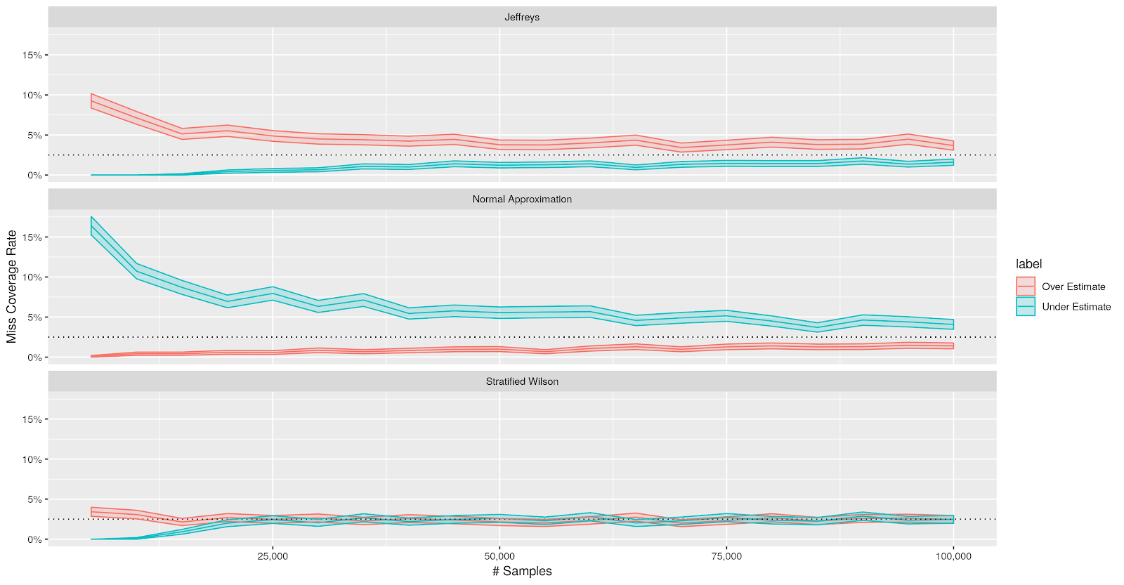 |
| Miss-coverage rate with 95% confidence bands. |
How Many Strata?
If post-stratification and stratified Wilson confidence interval can provide better uncertainty estimates, then it is natural to ask how many strata do we need. It really depends on the problem, but a rule of thumb is there should be enough positive and negative items in each stratum. If two strata do not have any positive items, with different sampling rates, merging them into a single strata without changing the number of samples will increase the effective sample size.There is an additional benefit of having coarse strata — it makes it harder for videos to move into different buckets when we retrain a new version of the classifier. This makes aggregating the metrics over multiple periods more robust, as we may sample items on different days with different versions of the classifier.
Cochran recommends no more than 6 or 7 strata [4] while others [5] suggest little to gained from going beyond 5 to 10 strata. Once you fix strata size, you might consider using the Danlenius-Hodges method [6] to select strata boundary.
Conclusion
In this post, we discussed the theory of importance sampling to improve the precision estimate of the binomial proportion of rare events. We also discuss how to design a sampling scheme and choose the appropriate aggregation metric to address practical concerns. The improvement of the metric depends on the precision/recall of the classifier, as well as many other factors. In our problem, when we apply post-stratification to importance sampling, we are able to more than triple the count positive items in the sample while reducing the CI width of the estimator by more than 30%. We hope you see similar gains in your application.References
[1] Art Owen. Unpublished book chapter on importance sampling.[2] Lawrence Brown, Tony Cai, Anirban DasGupta (2001). Interval Estimation for a Binomial Proportion. Statistical Science. 16 (2): 101–133.
[3] Xin Yan, Xiao Gang Su. Stratified Wilson and Newcombe Confidence Intervals for Multiple Binomial Proportions. Statistics in Biopharmaceutical Research, 2010.
[4] William Cochran (1977). Sampling Techniques pp 132-134.
[5] Ray Chambers, Robert Clark (2012). An Introduction to Model-Based Survey Sampling with Applications.
[6] Tore Dalenius, Joseph Hodges (1959). Minimum Variance Stratification. Journal of the American Statistical Association, 54, 88-101.
[7] Neyman, J. (1934). “On the Two Different Aspects of the Representative Method: The Method of Stratified Sampling and the Method of Purposive Selection”, Journal of the Royal Statistical Society, Vol. 97, 558-606.
[8] Tim Hesterberg (1995). Weighted Average Importance Sampling and Defensive Mixture Distributions. Technometrics, 37(2): 185 - 192.
Comments
Post a Comment