Customer Sentiments Analysis of Pepsi and Coca-Cola using Twitter Data in R
This article was published as a part of the Data Science Blogathon.
Introduction
Coca-Cola and PepsiCo are well-established names in the soft drink industry with both in the fortune 500. The companies that own a wide spectrum of product lines in a highly competitive market have a fierce rivalry with each other and constantly competing for market share in almost all subsequent product verticals.
We will analyze the sentiment of customers of these two companies with the help of 5000 tweets downloaded from each company’s official Twitter handle and analyzed in R. In this analysis, we will understand how we can customer sentiments from social media engagement of a brand (In this particular case tweeter).
Download the Twitter data here:
Contents
- Packages involved and their application
- What is Sentiment Analysis?
- Cleaning the text
- Word Cloud
- Distribution of tweets throughout the day and week
- Sentiment of tweets
- Emotional Analysis of customer’s tweets
- Conclusion
Packages used in R:
| Packages | Application |
| SentimentR | To calculate the numerical sentiment of a word. Its value can be negative or positive depending on the sentiment |
| Tm | Text mining package for text manipulation |
| Ggplot2 | To make graphs |
| Luberdate | To handle date and time |
| Worldcloud2 | To create a word cloud from text |
| Syuzhet | To convert dictionary words on a sentimental scale |
What is Sentiment Analysis?
Sentiment analysis is a text mining technique that provides context to the text and able to understand information from the subjective abstract source material, it helps in understanding social sentiment towards a brand product or service with the help of online conversation on a social media platform like Facebook, Instagram, and Twitter or via email. As we all are well aware that computers do not understand our general language, to make them understand the natural language we first convert the words into numerals format. With the help of an application, we will try to understand in a step by step manner.
Cleaning the text
As we have downloaded our dataset from Twitter which is mostly in the form of tweets, we all know the tweets contain links, hashtags, tweeter handle names, and emoticons in order to remove them we wrote function ions in R which I added below for your reference. After the removal of these, all text is converted to lower cases, removed stop words in the English language which have no meaning (like articles, prepositions, etc), punctuation, and numbers are also removed before converting them into a Document term Matrix.
Document term Matrix: is a Matrix that contains the count of how many times each word appears on each document, in our case tweets.
removeURL <- function(x) gsub(“(f|ht)tp(s?)://\S+”, “”, x, perl=T)
removeHashTags <- function(x) gsub(“#\S+”, “”, x)
removeTwitterHandles <- function(x) gsub(“@\S+”, “”, x)
removeSlash <- function(x) gsub(“n”,” “, x)
removeEmoticons <- function(x) gsub(“[^x01-x7F]”, “”, x)
data_pepsi$text <- iconv(data_pepsi$text, to = “utf-8”)
pepsi_corpus <- Corpus(VectorSource(data_pepsi$text))
pepsi_corpus <- tm_map(pepsi_corpus,tolower)
pepsi_corpus <- tm_map(pepsi_corpus,removeWords,stopwords(“en”))
pepsi_corpus <- tm_map(pepsi_corpus,content_transformer(removeHashTags))
pepsi_corpus <- tm_map(pepsi_corpus,content_transformer(removeTwitterHandles))
pepsi_corpus <- tm_map(pepsi_corpus,content_transformer(removeURL))
pepsi_corpus <- tm_map(pepsi_corpus,content_transformer(removeSlash))
pepsi_corpus <- tm_map(pepsi_corpus,removePunctuation)
pepsi_corpus <- tm_map(pepsi_corpus,removeNumbers)
pepsi_corpus <- tm_map(pepsi_corpus,content_transformer(removeEmoticons))
pepsi_corpus <- tm_map(pepsi_corpus,stripWhitespace)
pepsi_clean_df <- data.frame(text = get(“content”, pepsi_corpus))
dtm_pepsi <- DocumentTermMatrix(pepsi_corpus)
dtm_pepsi <- removeSparseTerms(dtm_pepsi,0.999)
pepsi_df <- as.data.frame(as.matrix(dtm_pepsi))
data_cola$text <- iconv(data_cola$text, to = “utf-8”)
cola_corpus <- Corpus(VectorSource(data_cola$text))
cola_corpus <- tm_map(cola_corpus,tolower)
cola_corpus <- tm_map(cola_corpus,removeWords,stopwords(“en”))
cola_corpus <- tm_map(cola_corpus,content_transformer(removeHashTags))
cola_corpus <- tm_map(cola_corpus,content_transformer(removeTwitterHandles))
cola_corpus <- tm_map(cola_corpus,content_transformer(removeURL))
cola_corpus <- tm_map(cola_corpus,content_transformer(removeSlash))
cola_corpus <- tm_map(cola_corpus,removePunctuation)
cola_corpus <- tm_map(cola_corpus,removeNumbers)
cola_corpus <- tm_map(cola_corpus,content_transformer(removeEmoticons))
cola_corpus <- tm_map(cola_corpus,stripWhitespace)
cola_clean_df <- data.frame(text = get(“content”, cola_corpus))
dtm_cola <- DocumentTermMatrix(cola_corpus)
dtm_cola <- removeSparseTerms(dtm_cola,0.999)
cola_df <- as.data.frame(as.matrix(dtm_cola))
Word Cloud
Word cloud is a representation of test data that highlights the most frequent words by increasing the size of it. The technique is used to visualize text as an image. It is a collection of words or tags. In R it can be made using worldcloud2 package. The following are the codes for it with output
word_pepsi_df <- data.frame(names(pepsi_df),colSums(pepsi_df))
names(word_pepsi_df) <- c(“words”,”freq”)
word_pepsi_df <- subset(word_pepsi_df, word_pepsi_df$freq > 0)
wordcloud2(data = word_pepsi_df,size = 1.5,color = “random-light”,backgroundColor = “dark”)
word_cola_df <- data.frame(names(cola_df),colSums(cola_df))
names(word_cola_df) <- c(“words”,”freq”)
word_cola_df <- subset(word_cola_df, word_cola_df$freq > 0)
wordcloud2(data = word_cola_df,size = 1.5,color = “random-light”,backgroundColor = “dark”)
Wordcloud of tweets for Pepsi and Coca-Cola
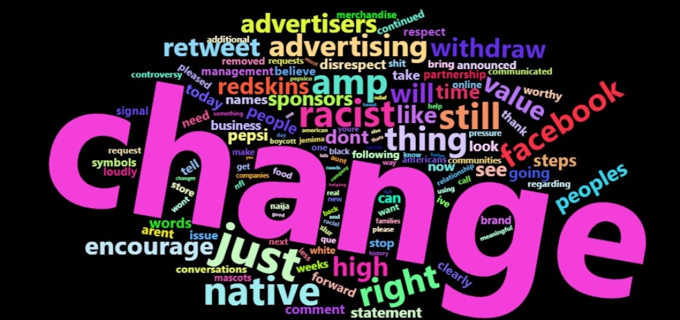
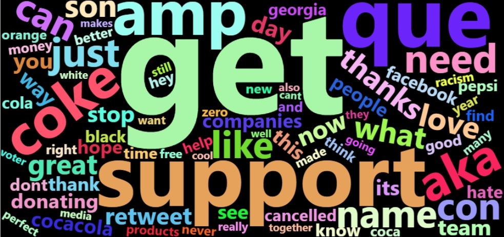
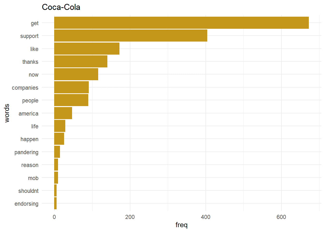
As we know word size in a word cloud is subject to its frequency in the tweets, so words live the change, just, native, right, racism is prevalent while words like getting and support appear more in tweets from customers of Coca-Cola.
Distribution of tweets throughout the day and week
As the tweets were collected for a time span of over a week, we can analyze the hours and weekdays which have most users active or users tweeting most about the brand. This can be visualized using a line chart using a library ggplot2. Below are the function used with the output
data_pepsi$Date <- as.Date(data_pepsi$created_at)
data_pepsi$hour <- hour(data_pepsi$created_at)
data_pepsi$weekday<-factor(weekdays(data_pepsi$Date),levels=c(“Monday”,”Tuesday”,”Wednesday”,”Thursday”,”Friday”,”Saturday”,”Sunday”))
ggplot(data_pepsi,aes(x= hour)) + geom_density() + theme_minimal() + ggtitle(“Pepsi”)
ggplot(data_pepsi,aes(x= weekday)) + geom_bar(color = “#CC79A7”, fill = “#CC79A7”) + theme_minimal() +ggtitle(“Pepsi”) + ylim(0,1800)
data_cola$Date <- as.Date(data_cola$created_at)
data_cola$Day <- day(data_cola$created_at)
data_cola$hour <- hour(data_cola$created_at)
data_cola$weekday<-factor(weekdays(as.Date(data_cola$Date)),levels=c(“Monday”,”Tuesday”,”Wednesday”,”Thursday”,”Friday”,”Saturday”,”Sunday”))
ggplot(data_cola,aes(x= hour)) + geom_density() + theme_minimal() + ggtitle(“Coca-Cola”)
ggplot(data_cola,aes(x=
weekday)) + geom_bar(color = “#CC79A7”, fill = “#CC79A7”) + theme_minimal()
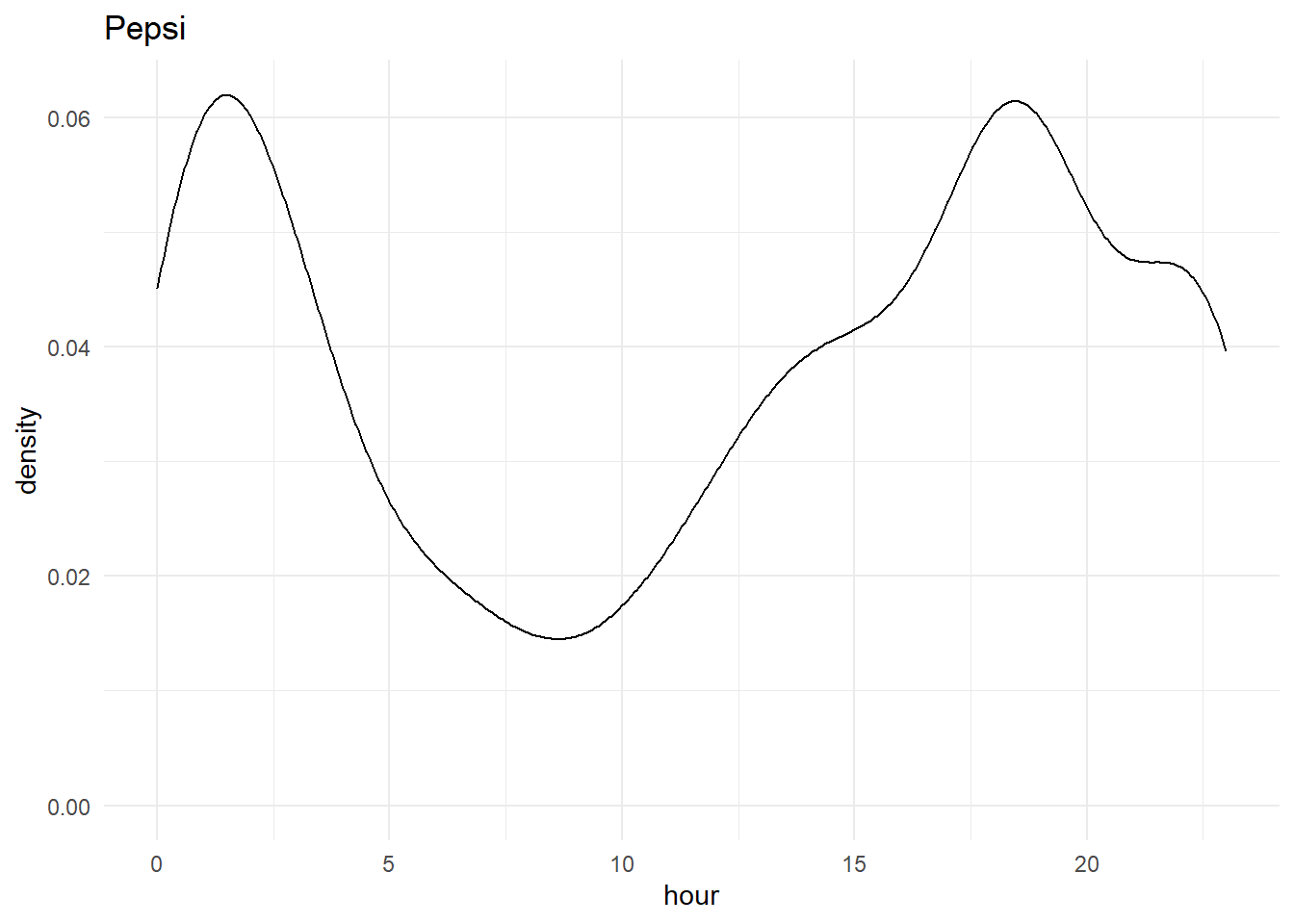
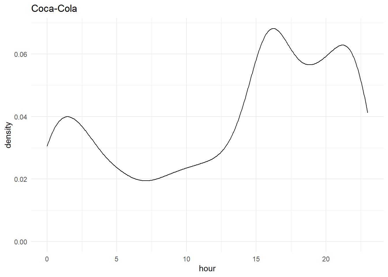
From the above graphs, we can see a spike in both Pepsi and Coca-cola during 3-4 pm and around 1 am as people like to use more social media when they are bored at work or late at night which is quite evident from our analysis
Distribution of tweets throughout the week
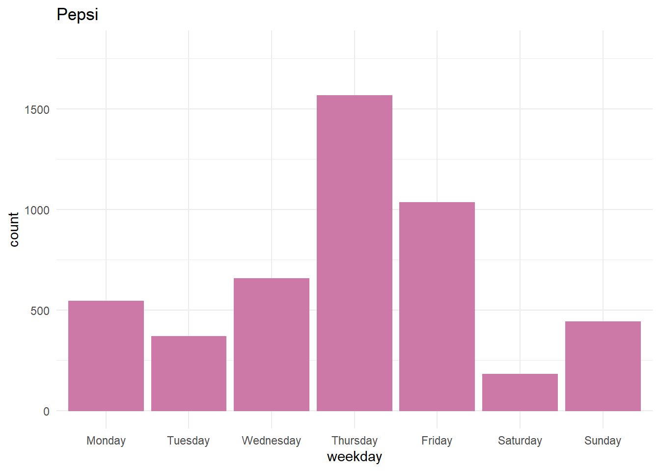
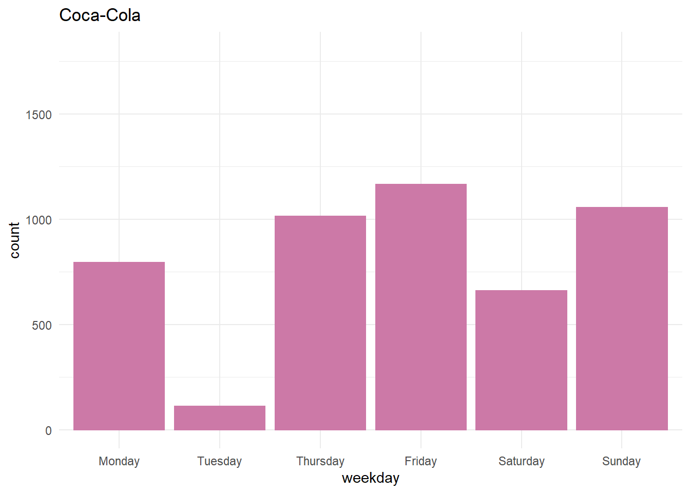
When daily tweets are shown on the bar-graph. For Pepsi, Thursday was the day with the most number of tweets which is due to the fact that they published their quarter reports (at the time of downloading tweets). But in the case of Coca-Cola on Tuesday we saw the least number of tweets.
Sentiment of tweets
In this section, tweets are categorized into positive-negative, and neutral. This is achieved with the help of sentimentR package which assigns a sentiment score from -1 to +1 to each dictionary word and taking an average of each word in the tweet, the final sentiment score of each tweet is obtained.
sentiments <- sentiment_by(get_sentences(pepsi_clean_df$text))
data$sentiment_score <- round(sentiments$ave_sentiment,2)
data$sentiment_score[data_pepsi$sentiment_score > 0] <- “Positive”
data$sentiment_score[data_pepsi$sentiment_score < 0] <- “Negative”
data$sentiment_score[data_pepsi$sentiment_score == 0] <- “Neutral”
data$sentiment_score <- as.factor(data$sentiment_score)
ggplot(data,aes(x = sentiment_score)) + geom_bar(color = “steelblue”, fill = “steelblue”) + theme_minimal()
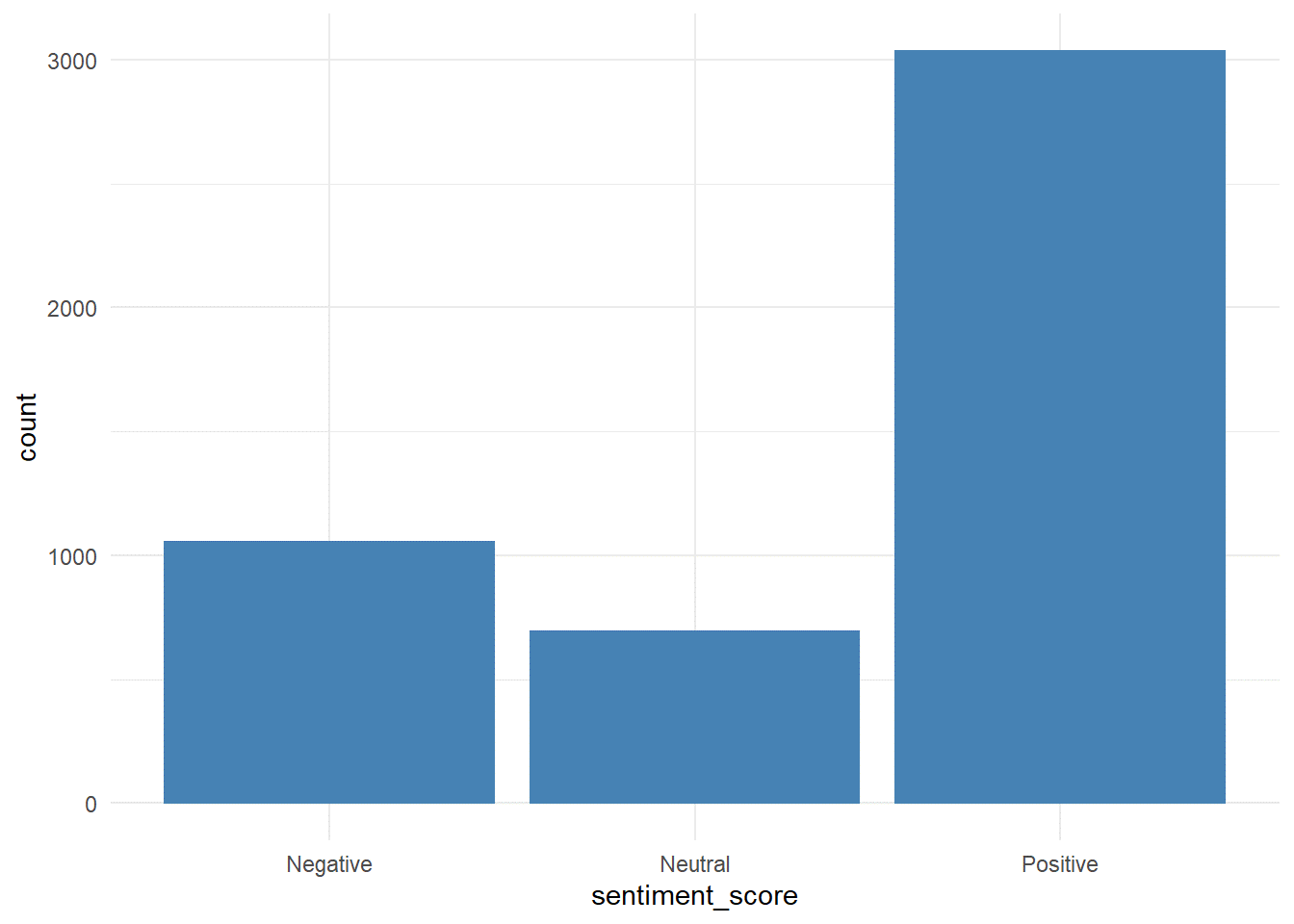
Sentiments of almost 75 percent of tweets are positive as we all know these two brands are quite popular among their customers.
Emotional Analysis of customer’s tweets
Emotions of a tweet are performed by Syuzhet package which rates each dictionary word on a ten emotion index which includes anger, anticipation, disgust, fear, joy, sadness, surprise, trust, negative and positive. If we sum up the values of each word on the index. The emotional sentiment of all tweets can be presented on a bar graph.
cols <- c(“red”,”pink”,”green”,”orange”,”yellow”,”skyblue”,”purple”,”blue”,”black”,”grey”)
pepsi_sentimentsdf <- get_nrc_sentiment(names(pepsi_df))
barplot(colSums(pepsi_sentimentsdf),
main = “Pepsi”,col = cols,space = 0.05,horiz = F,angle = 45,cex.axis = 0.75,las = 2,srt = 60,border = NA)
cola_sentimentsdf <- get_nrc_sentiment(names(cola_df))
barplot(colSums(cola_sentimentsdf),
main = “Coca-Cola”,col = cols,space = 0.05,horiz = F,angle = 45,cex.axis = 0.75,las = 2,srt = 60,border = NA)
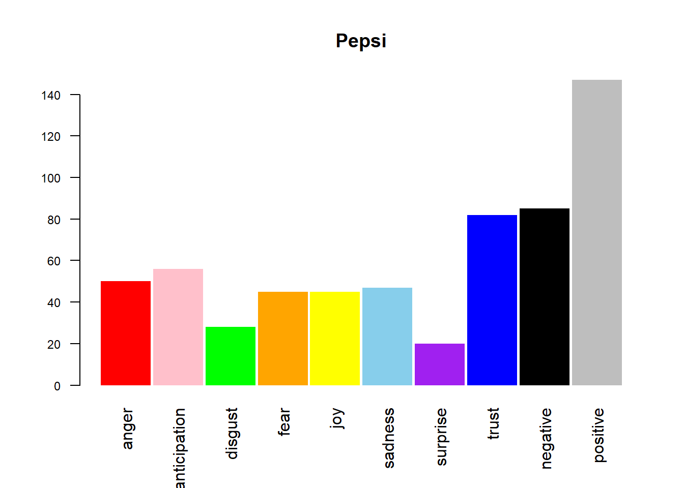
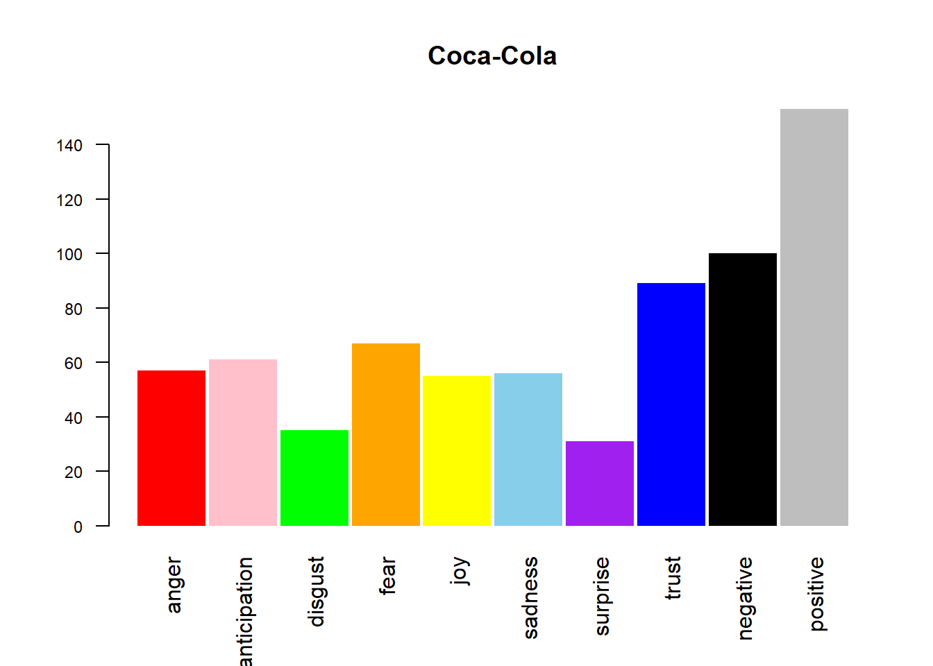
The above output is the display of all the emotion on a barplot of as it is quite clear from the barplot that positivity dominates for both the companies which further strengthens our above hypothesis. Continue tracking the changes in the graph can act as feedback towards a new product or an advertisement.
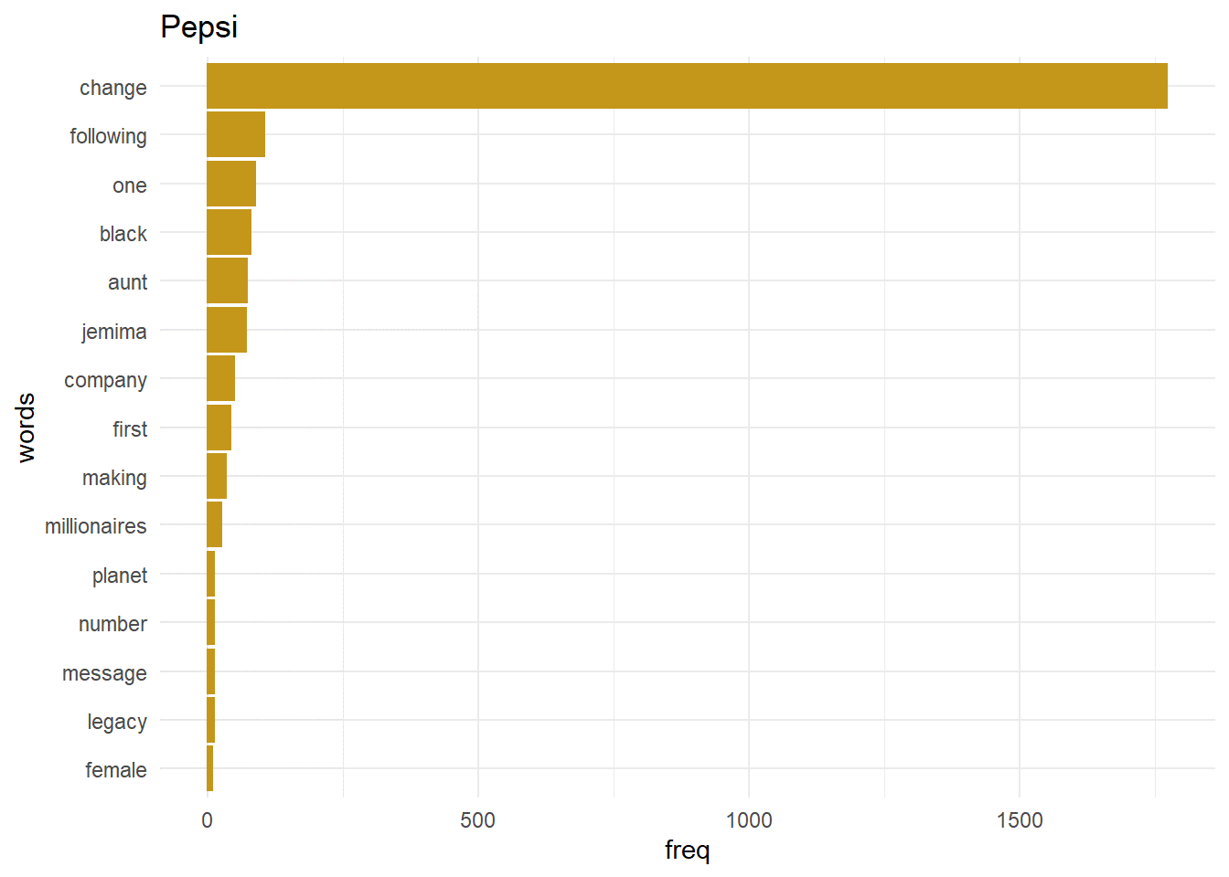
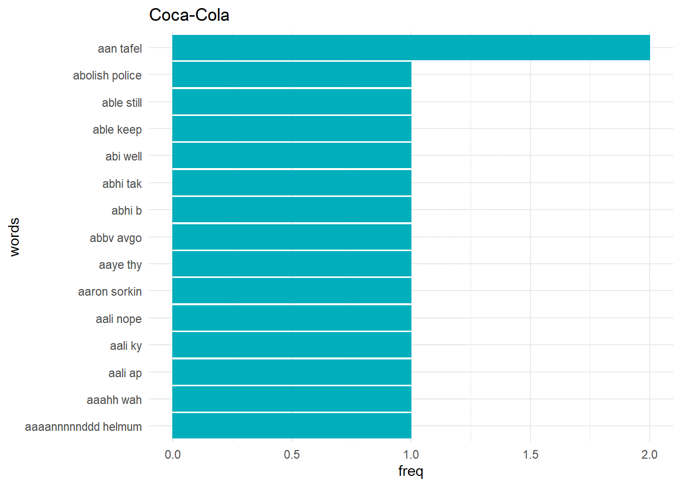
Most frequent words
word_pepsi_df$words <- factor(word_pepsi_df$words, levels = word_pepsi_df$words[order(word_pepsi_df$freq)])
word_cola_df$words <- factor(word_cola_df$words, levels = word_cola_df$words[order(word_cola_df$freq)])
ggplot(word_pepsi_df[1:15,],aes(x = freq, y = words)) + geom_bar(stat = “identity”, color = “#C4961A”,fill = “#C4961A”) + theme_minimal() + ggtitle(“Pepsi”)
ggplot(word_cola_df[1:15,],aes(x = freq, y = words)) + geom_bar(stat = “identity”, color = “#C4961A”,fill = “#C4961A”) + theme_minimal() + ggtitle(“Coca-Cola”)
createNgram <-function(stringVector, ngramSize){
ngram <- data.table()
ng <- textcnt(stringVector, method = “string”, n=ngramSize, tolower = FALSE)
if(ngramSize==1){
ngram <- data.table(w1 = names(ng), freq = unclass(ng), length=nchar(names(ng)))
}
else {
ngram <- data.table(w1w2 = names(ng), freq = unclass(ng), length=nchar(names(ng)))
}
return(ngram)
}
pepsi_bigrams_df <- createNgram(pepsi_clean_df$text,2)
cola_bigrams_df <- createNgram(cola_clean_df$text,2)
pepsi_bigrams_df$w1w2 <- factor(pepsi_bigrams_df$w1w2,levels = pepsi_bigrams_df$w1w2[order(pepsi_bigrams_df$freq)])
cola_bigrams_df$w1w2 <- factor(cola_bigrams_df$w1w2,levels = cola_bigrams_df$w1w2[order(cola_bigrams_df$freq)])
names(pepsi_bigrams_df) <- c(“words”, “freq”, “length”)
names(cola_bigrams_df) <- c(“words”, “freq”, “length”)
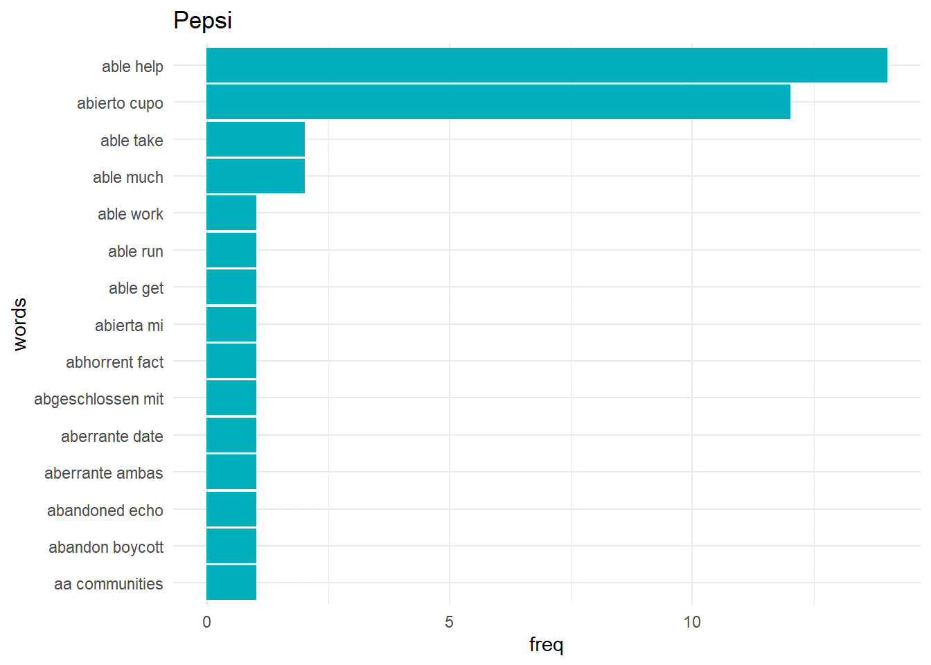
ggplot(pepsi_bigrams_df[1:15,],aes(x = freq, y = words)) + geom_bar(stat = “identity”, color = “#00AFBB”,fill = “#00AFBB”) + theme_minimal() + ggtitle(“Pepsi”)
ggplot(cola_bigrams_df[1:15,],aes(x = freq, y = words)) + geom_bar(stat = “identity”, color = “#00AFBB”,fill = “#00AFBB”) + theme_minimal() + ggtitle(“Coca-Cola”)
Bigrams
Bigrams are pair of words which are created when the sentences are broken two words at a time. It is beneficial to get the context of the word as a single word generally doesn’t provide any context.
Conclusion
As we can see that from the available social media engagement companies can analyze the sentiments of their customers and create business strategies accordingly. The above analysis can be used to see the direct impact of a companies decision say launching of a product line.
The media shown in this article are not owned by Analytics Vidhya and is used at the Author’s discretion.


Good paper, thank you! Could you please tell the data source? It is not included. Thanks: peter
Thank you for the nice paper. Could you please send a link to the dataset if available.
Hello Peter, Thanks for the appreciation. The website won't allow me to post the link to my dataset, so can you give me your email?
Hi! Your paper was amazing. Can I request for the datasets? It is for my thesis and it will be a big help for ny study. Have a nice day
i request for the data. kindly reach out