A simple start with Natural Language Processing!
This article was published as a part of the Data Science Blogathon
Introduction to NLP:
After I got acquainted with Machine learning concepts, I was wary of venturing into NLP. To me, NLP was a subject area posing a complicated outlook. But after my first encounter with it, I have come to realize that though it is hard to master it, it is easy to follow the concepts.
I am presenting some basic NLP concepts and their work.
NLP or Natural Language Processing is how machine understands and deals with human languages. Language processing implies text data that is unstructured.
Data availability and synthetic data generation are complexities involved in general with any type of machine learning use cases. But the NLP is the field where that problem is relatively less pronounced, as there are a lot of text data around us – the emails we write, the comments we post, blogs we write, etc.,
Types:
Some of its types are-
1) Named entity recognition – the process of extracting keywords/nouns (names entities) in the text, thus extracting useful information from the text, that can be used for various purposes like classification, recommendation, sentiment analysis, etc. A chatbot is the most common use case. The query of the user is understood through the entities in the text and responded with accordingly.
2) Text summarization – is where key concepts of the huge text is extracted and paraphrased summary is built around it. This can be instrumental in the use cases of large search results.
3) Translation – understand the text in 1 language and translate it to another language. Google translator is the most common example here.
4) Speech to text – converts speech to text data, the most common example being assistants in our Smartphones.
5) NLU – Natural Language Understanding is a way of understanding the words and sentences with respect to the context. These are helpful in sentiment analysis of the review comments of users/consumers.
6) NLG – Natural Language Generation goes beyond machine processing or comprehending the text. This is the ability of the machines to write content by themselves. A highly advanced GTP-3 transformer deep net wrote this article.
These areas can be found overlapping based on the use cases.
A simple start:
The insights into how Machine Learning deals with unstructured text data is presented through a basic example of text classification.
Input:
A ‘text’ column with review comments by user
A ‘label’ column with a flag to denote if it is a positive or a negative comment.
Output:
The task is to classify the comments based on the sentiment as positive or negative.
Preprocessing steps:
Some preprocessing will be made to get the data ready for ML algorithms. As text cannot be directly dealt with by machines, it is converted to numbers. This way, unstructured data is converted to structured data.
NLTK is a python library that aids NLP use cases and caters very well for our preprocessing needs.
1) Stop words removal:
Stop words occur frequently and do not add much meaning to the text. Search engines are also programmed to ignore the stop words. Sample stop words are – of, the, it, has, his, what, etc
Removing stop words help the code concentrate on the main keywords of the text that add more to the context.
Explanation code:
Implementation code:
Applying stop words removal to a pandas dataframe with a ‘text’ column
input_df[‘text’] = input_df[‘text’].apply(lambda x: “ “.join(x for x in x.split() if x not in stop))
2) Emojis and special characters removal:
User comments are laden with emojis and special characters. These characters are represented as Unicode characters in text, denoted as U+, ranging from U+0000 to U+10FFFF
Sample code(reference code):
import re
def remove_emoji(text):
        emoji_pattern = re.compile("["
        u"U0001F600-U0001F64F"  # emoticons
        u"U0001F300-U0001F5FF"  # symbols & pictographs
        u"U0001F680-U0001F6FF"  # transport & map symbols
        u"U0001F1E0-U0001F1FF"  # flags (iOS)
        u"U0001F1F2-U0001F1F4"  # Macau flag
        u"U0001F1E6-U0001F1FF"  # flags
        u"U0001F600-U0001F64F"
        u"U00002702-U000027B0"
        u"U000024C2-U0001F251"
        u"U0001f926-U0001f937"
        u"U0001F1F2"
        u"U0001F1F4"
        u"U0001F620"
        u"u200d"
        u"u2640-u2642"
        "]+", flags=re.UNICODE)
return emoji_pattern.sub(r'', text)
sample_text= 'That was very funny 😂. Have a lovely day 💕 '
remove_emoji(sample_text)
Output:
‘That was very funny . Have a lovely day ‘
Implementation code:
input_df[‘text’] = input_df[‘text’].apply(lambda x: remove_emoji(x))
3) Inflection:
Inflection is the modification of a word to express different grammatical categories such as tense, case, voice, aspect, person, number, gender and mood. For instance, inflections of ‘come’ are ‘came’, ‘comes’. To get the best result, the inflections of a word have to treated in the same way. To handle inflection stemming and lemmatization can be used.
Stemming and lemmatization work on words. So, the text is tokenized into words before applying them. The resultant words are then combined back to the sentence and returned.
1) Stemming:
Stemming is a rule-based approach that converts the words to their root word (stem) to remove the inflection without worrying about the context of the word in the sentence. This is used when the meaning of the word is not important. The stemmed word might be a meaningless word in itself.
Explanation code:
from nltk.stem import PorterStemmer
porter = PorterStemmer()
Sample 1:
print(porter.stem('trembling'),
porter.stem('tremble'),
porter.stem('trembly'))
Output:
trembl trembl trembl
Sample 2:
print(porter.stem('study'),
porter.stem('studying'),
porter.stem('studies'))
Output:
studi studi studi
Implementation code:
def stemming_text(text):
    stem_words = [porter.stem(w) for w in w_tokenizer.tokenize(text)]
    return ‘ ‘.join(stem_words)
input_df[‘text’] = input_df[‘text’].apply(lambda x: stemming_text(x))
2) Lemmatization:
Lemmatization, unlike Stemming, reduces the inflected words properly ensuring that the root word (lemma) belongs to the language. Though lemmatization is slower compared to stemming, it considers the context of the word by taking into account the preceding word, which results in better accuracy.
Explanation code:
w_tokenizer = nltk.tokenize.WhitespaceTokenizer()
lemmatizer = nltk.stem.WordNetLemmatizer()
def lemmatize_text(text):
    lemma_words = [lemmatizer.lemmatize(w) for w in w_tokenizer.tokenize(text)]
    return ‘ ‘.join(lemma_words)
print(lemmatize_text('study'),
     lemmatize_text('studying') ,
     lemmatize_text('studies'))
Output:
study studying study
print(lemmatize_text('trembling'),
     lemmatize_text('tremble') ,
     lemmatize_text('trembly'))
Output:
trembling tremble trembly
Implementation code:
input_df[‘text’] = input_df[‘text’].apply(lemmatize_text)
4) Vectorizer
This is the step where the words are converted to numbers, which can be processed by the algorithms.
These resultant numbers are in the vectors form, hence the name.
1) Bag of words model:
This is the most basic of vectorizers. The vector formed has words in the text and their frequency. It is as if the words are put in a bag. The order of the words is not retained.
Explanation code:
from sklearn.feature_extraction.text import CountVectorizer
bagOwords = CountVectorizer()
print(bagOwords.fit_transform(text).toarray())
print('Features:', bagOwords.get_feature_names())
Input:
text = [“I like the product very much. The quality is very good.”,
“The product is very very good”,
“Broken product delivered”,
“The product is good, but overpriced product”,
“The product is not good”]
Output:
array([[0, 0, 0, 1, 1, 1, 1, 0, 0, 1, 1, 2, 2],
[0, 0, 0, 1, 1, 0, 0, 0, 0, 1, 0, 1, 1],
[1, 0, 1, 0, 0, 0, 0, 0, 0, 1, 0, 0, 0],
[0, 1, 0, 1, 1, 0, 0, 0, 1, 2, 0, 1, 0],
[0, 0, 0, 1, 1, 0, 0, 1, 0, 1, 0, 1, 0]])
Features: [‘broken’, ‘but’, ‘delivered’, ‘good’, ‘is’, ‘like’, ‘much’, ‘not’, ‘overpriced’, ‘product’, ‘quality’, ‘the’, ‘very’]
Comments 2 and 5 are not very different in the result, however, the sentiment they convey are opposite. The returned matrix is sparse.
2) n-grams:
Unlike the bag of words approach, the n-gram approach relies on the order of the words to derives their context. n-gram is a contiguous sequence of n-items in a text. So the feature set built using the n-grams feature will have n number of consecutive words as features. The value for n can be given as a range.
Explanation code:
count_vec = CountVectorizer(analyzer='word', ngram_range=(1, 2))
print('Features:', count_vec.get_feature_names())
print(count_vec.fit_transform(text).toarray())
Output:
[[0 0 0 0 0 1 0 1 0 0 1 1 1 1 1 0 0 0 0 1 0 0 1 1 1 2 1 1 2 1 1] [0 0 0 0 0 1 0 1 0 0 1 0 0 0 0 0 0 0 0 1 0 1 0 0 0 1 1 0 1 1 0] [1 1 0 0 1 0 0 0 0 0 0 0 0 0 0 0 0 0 0 1 1 0 0 0 0 0 0 0 0 0 0] [0 0 1 1 0 1 1 1 1 0 0 0 0 0 0 0 0 1 1 2 0 1 0 0 0 1 1 0 0 0 0]
[0 0 0 0 0 1 0 1 0 1 0 0 0 0 0 1 1 0 0 1 0 1 0 0 0 1 1 0 0 0 0]]
Features: [‘broken’, ‘broken product’, ‘but’, ‘but overpriced’, ‘delivered’, ‘good‘, ‘good but’, ‘is’, ‘is good’, ‘is not’, ‘is very’, ‘like’, ‘like the’, ‘much’, ‘much the’, ‘not’, ‘not good’, ‘overpriced’, ‘overpriced product’, ‘product’, ‘product delivered’, ‘product is’, ‘product very’, ‘quality’, ‘quality is’, ‘the’, ‘the product’, ‘the quality’, ‘very’, ‘very good’, ‘very much’]
3) TF-IDF:
Just because a word appears with high frequency does not suggest that the word adds a significant effect on the sentiment that we are looking for. The word may be common across all the sample texts/documents. For instance, the word ‘product’ in our sample is redundant and does not give much information related to the sentiment. It only adds to the feature-length.
Term frequency(TF) – is the frequency of the words in a sample text.
Inverse Document Frequency(IDF) – highlights the frequency of the words across other samples texts. The features are rare or common across the sample texts is the key concern here.
When we use both TF-IDF together(TF*IDF), the high-frequency words in a sample text that has low occurrence in other sample texts are given higher importance.
Explanation code:
from sklearn.feature_extraction.text import TfidfVectorizer
tf_idf_vec = TfidfVectorizer(use_idf=True,
                        smooth_idf=False,
                        ngram_range=(1,1))
print(tf_idf_vec.fit_transform(text).toarray())
print('Features:', tf_idf_vec.get_feature_names())
Output:
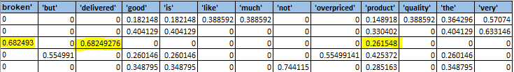
In the third sample text, the values words ‘broken’ and ‘delivered’ are rare across all texts and are given higher score than ‘product’ which is a recurring word.
Implementation code:
                    tfidf_vec = TfidfVectorizer(use_idf=True)
                    tfidf_vec.fit(input_df[‘text’])
                    tfidf_result = tfidf_vec.transform(input_df[‘text’])
5) Class imbalance:
Mostly this kind of scenario will have a class imbalance. The text data would include more positive sentiment cases than negative ones. The simplest way of handling class imbalance is by augmenting data with exact copies of the minority class (in our
case the negative sentiment scenarios). This technique is called oversampling.
Machine learning algorithm:
After the processing steps are complete, the data is ready to be passed into a machine learning algorithm for fitting and prediction. This is an iterative process in which a suitable algorithm is chosen and hyperparameter tuning is done.
A point to note here is that apparently, like any other ML problem, the preprocessing steps have to be handled after the train and test split.
Implementation code:
from sklearn.ensemble import RandomForestClassifier
from sklearn.metrics import f1_score
rnd_mdl = RandomForestClassifier()
rnd_mdl.fit(tfidf_result, input_df[‘label’])
#Using the fitted model to predict from the test data
#test_df is the test data and tfidf_result_test is the preprocessed test text data
output_test_pred = rnd_mdl.predict(tfidf_result_test)
#finding f1 score for the generated model
test_f1_score = f1_score(test_df[‘label’], output_test_pred)
Prebuilt library:
There is a prebuilt library in NLTK that scores the text data based on sentiment. It does not need these preprocessing steps. It is called nltk.sentiment.SentimentAnalyzer
Endnotes:
There are plenty of advanced pre-trained deep learning models available for NLP. The preprocessing involved when using these deep nets vary considerably from the ML approach given here.
This is a simple introduction to the interesting NLP world! It is a vast space that is continuously evolving. Well begun is half done!


