A Hands-on Guide to Build Your First Convolutional Neural Network Model
This article was published as a part of the Data Science Blogathon
Overview
This article will briefly discuss CNNs, a special variant of neural networks designed specifically for image-related tasks. The article will mainly focus on the implementation part of CNN. Maximum efforts have been made to make this article interactive and simple. Hope you enjoy it.Happy learning!!
Introduction
Convolutional Neural networks were introduced by Yann LeCun and Yoshua Bengio in the year 1995 which later proved to show exceptional results in the domain of images. So what made them special compared to the ordinary neural networks when applied in the image domain? I will explain one of the reasons with a simple example. Consider that you are given the task of classifying the images of handwritten digits and given below are some samples from training sets.
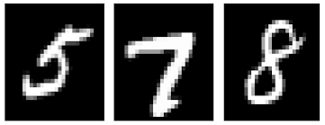
If you properly observe you can find that all the digits are occurring at the centre of the respective images. Training a normal neural network model with these images may give a good result if the test image is of a similar type. But what if the test image is like the one shown below?

Here number nine appears in the corner of the image. If we use a simple neural network model to classify this image, our model may fail abruptly. But if the same test image is given to a CNN model, chances are high that it will classify correctly. The reason for the better performance is that it looks for spatial features in the image. For the above case itself, even if the number nine lies in the left corner of the frame, the trained CNN model captures the features in the image and most probably predicts that the number is the digit nine. A normal neural network can’t do this kind of magic. Now let’s discuss briefly discuss the main building blocks of CNN.
Main components in the architecture of a CNN model
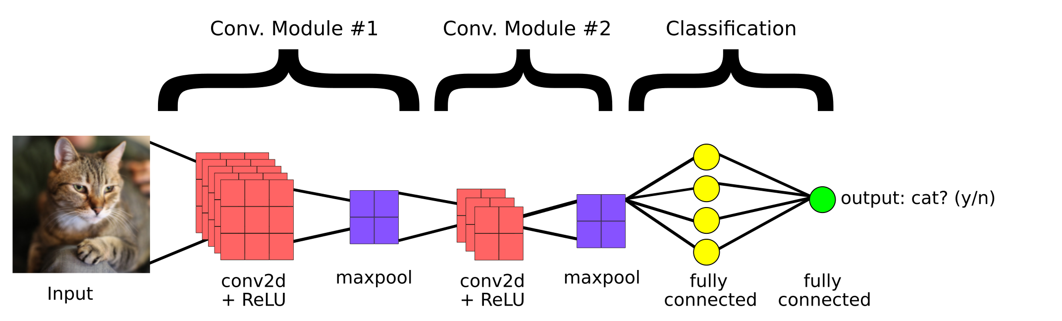
This is a simple CNN model built to classify whether the image contains a cat or not. So, the main components of a CNN are:
1. Convolutional Layer
2. Pooling Layer
3.Fully Connected Layer
Convolutional Layer
Convolutional Layers help us to extract the features that are present in the image. This extraction is achieved with the help of filters. Please observe the below operation.
Here we can see that a window is sliding over the entire image where the image is represented as a grid (That’s the way the computer sees images where the grides are filled with numbers!). Now let’s see how the calculations take place in the convolution operation.
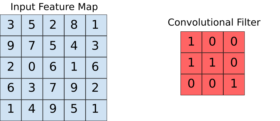
Assume that the input feature map is our image and the convolutional filter is the window that we are going to slide over. Now let us observe one of the instances of the convolution operation.

When the convolution filter is superimposed over the image, the respective elements are getting multiplied. The multiplied values are then summed together to get a single value that is filled in the output feature map. This operation is continued until we slide the window all over the input feature map thereby filling the output feature map.
Pooling Layer
The idea behind using a pooling layer is to reduce the dimension of the feature map. For the representation given below, we have used a 2*2 max-pooling layer. Each time the window slides over the image, we take the maximum value present inside the window.
Finally, after the max pool operation, we can see here that the dimension of the input i.e. 4*4 has been scaled down to 2*2.
Fully Connected Layer
This layer is present at the tail section of the CNN model architecture as seen before. The input to the fully connected layer is the rich features that have been extracted using convolutional filters. This is then forward propagated till the output layer, where we get the probability of the input image belonging to different classes. The predicted output is the class with the highest probability that the model has predicted.
Code Implementation
Here we are taking the Fashion MNIST as our problem dataset. The dataset contains T-shirts, trousers, pullovers, dresses, coats, sandals, shirts, sneakers, bags, and ankle boots. The task is to classify a given image into the above-mentioned classes after training the model.
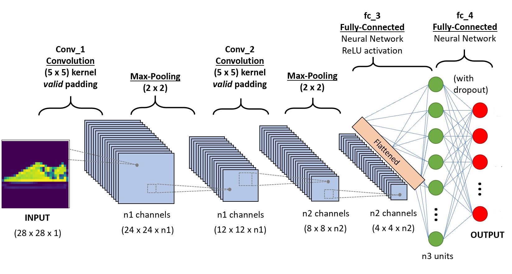
We will implement the code in Google Colab as they provide the usage of free GPU resources for a fixed period of time. If you are new to the Colab environment and GPUs, please check out this blog to get a better idea. Given below is the architecture of the CNN that we are going to build.
Step-1: Importing the necessary libraries
import os
import torch
import torchvision
import tarfile
from torchvision import transforms
from torch.utils.data import random_split
from torch.utils.data.dataloader import DataLoader
import torch.nn as nn
from torch.nn import functional as F
from itertools import chain
Step -2: Downloading the train and test Dataset
train_set = torchvision.datasets.FashionMNIST("/usr", download=True, transform=
                                                transforms.Compose([transforms.ToTensor()]))
test_set = torchvision.datasets.FashionMNIST("./data", download=True, train=False, transform=
                                               transforms.Compose([transforms.ToTensor()]))
Step-3 Splitting the training set to train and validation
train_size = 48000
val_size = 60000 - train_size
train_ds,val_ds = random_split(train_set,[train_size,val_size])
Step-4 Loading the dataset into memory using Dataloader
train_dl = DataLoader(train_ds,batch_size=20,shuffle=True)
val_dl = DataLoader(val_ds,batch_size=20,shuffle=True)
classes = train_set.classes
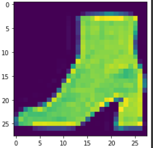
Now let us visualize the loaded data,
for imgs,labels in train_dl:
  for img in imgs:
    arr_ = np.squeeze(img)
    plt.show()
    break
  break
Step -5 Defining the architecture
import torch.nn as nn
import torch.nn.functional as F
#define the CNN architecture
class Net(nn.Module):
    def __init__(self):
        super(Net, self).__init__()
        #convolutional layer-1
        self.conv1 = nn.Conv2d(1,6,5, padding=0)
        #convolutional layer-2
        self.conv2 = nn.Conv2d(6,10,5,padding=0)
        # max pooling layer
        self.pool = nn.MaxPool2d(2, 2)
        # Fully connected layer 1
        self.ff1 = nn.Linear(4*4*10,56)
        # Fully connected layer 2
        self.ff2 = nn.Linear(56,10)
    def forward(self, x):
        # adding sequence of convolutional and max pooling layers
        #input dim-28*28*1
        x = self.conv1(x)
        # After convolution operation, output dim - 24*24*6
        x = self.pool(x)
        # After Max pool operation output dim - 12*12*6
        x = self.conv2(x)
        # After convolution operation  output dim - 8*8*10
        x = self.pool(x)
        # max pool output dim 4*4*10
        x = x.view(-1,4*4*10) # Reshaping the values to a shape appropriate to the input of fully connected layer
        x = F.relu(self.ff1(x)) # Applying Relu to the output of first layer
        x = F.sigmoid(self.ff2(x)) # Applying sigmoid to the output of second layer
        return x
# create a complete CNN
model_scratch = Net()
print(model)
# move tensors to GPU if CUDA is available
if use_cuda:
    model_scratch.cuda()
Step 6 – Defining the loss function
# Loss function
import torch.nn as nn
import torch.optim as optim
criterion_scratch = nn.CrossEntropyLoss()
def get_optimizer_scratch(model):
    optimizer = optim.SGD(model.parameters(),lr = 0.04)
    return optimizer
Step 7 – Implementing the training and validation algorithm
# Implementing the training algorithm
def train(n_epochs, loaders, model, optimizer, criterion, use_cuda, save_path):
    """returns trained model"""
    # initialize tracker for minimum validation loss
    valid_loss_min = np.Inf
    for epoch in range(1, n_epochs+1):
        # initialize variables to monitor training and validation loss
        train_loss = 0.0
        valid_loss = 0.0
        # train phase #
        # setting the module to training mode
        model.train()
        for batch_idx, (data, target) in enumerate(loaders['train']):
            # move to GPU
            if use_cuda:
                data, target = data.cuda(), target.cuda()
            optimizer.zero_grad()
            output = model(data)
            loss = criterion(output, target)
            loss.backward()
            optimizer.step()
            train_loss = train_loss + ((1 / (batch_idx + 1)) * (loss.data.item() - train_loss))
        # validate the model #
        # set the model to evaluation mode
        model.eval()
        for batch_idx, (data, target) in enumerate(loaders['valid']):
            # move to GPU
            if use_cuda:
                data, target = data.cuda(), target.cuda()
            output = model(data)
            loss = criterion(output, target)
            valid_loss = valid_loss + ((1 / (batch_idx + 1)) * (loss.data.item() - valid_loss))
# print training/validation statistics
        print('Epoch: {} tTraining Loss: {:.6f} tValidation Loss: {:.6f}'.format(
            epoch,
            train_loss,
            valid_loss
            ))
## If the valiation loss has decreased, then saving the model
        if valid_loss <= valid_loss_min:
            print('Validation loss decreased ({:.6f} --> {:.6f}).  Saving model ...'.format(
            valid_loss_min,
            valid_loss))
            torch.save(model.state_dict(), save_path)
            valid_loss_min = valid_loss
    return model
Step-8: Training and evaluation phase
num_epochs = 15
model_scratch = train(num_epochs, loaders_scratch, model_scratch, get_optimizer_scratch(model_scratch),
                      criterion_scratch, use_cuda, 'model_scratch.pt')
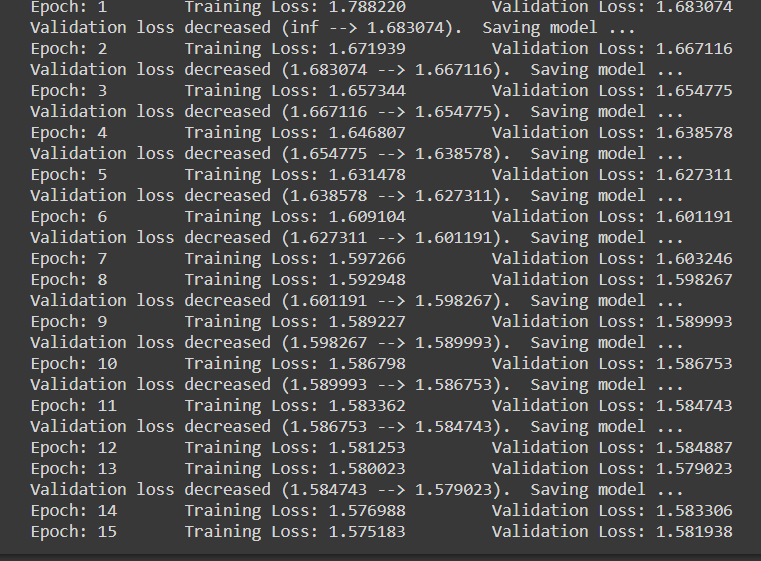
Note that when each time the validation loss is decreasing, we are saving the state of the model.
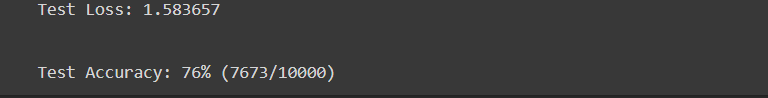
Step- 9 Testing Phase
def test(loaders, model, criterion, use_cuda):
# monitor test loss and accuracy
    test_loss = 0.
    correct = 0.
    total = 0.
# set the module to evaluation mode
    model.eval()
    for batch_idx, (data, target) in enumerate(loaders['test']):
          # move to GPU
          if use_cuda:
            data, target = data.cuda(), target.cuda()
          # forward pass: compute predicted outputs by passing inputs to the model
          output = model(data)
          # calculate the loss
          loss = criterion(output, target)
          # update average test loss
          test_loss = test_loss + ((1 / (batch_idx + 1)) * (loss.data.item() - test_loss))
          # convert output probabilities to predicted class
          pred = output.data.max(1, keepdim=True)[1]
          # compare predictions to true label
        correct += np.sum(np.squeeze(pred.eq(target.data.view_as(pred)),axis=1).cpu().numpy())
        total += data.size(0)
 print('Test Loss: {:.6f}n'.format(test_loss))
print('nTest Accuracy: %2d%% (%2d/%2d)' % (
        100. * correct / total, correct, total))
# load the model that got the best validation accuracy
model_scratch.load_state_dict(torch.load('model_scratch.pt'))
test(loaders_scratch, model_scratch, criterion_scratch, use_cuda)
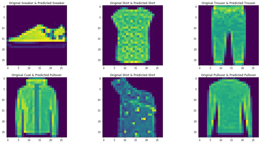
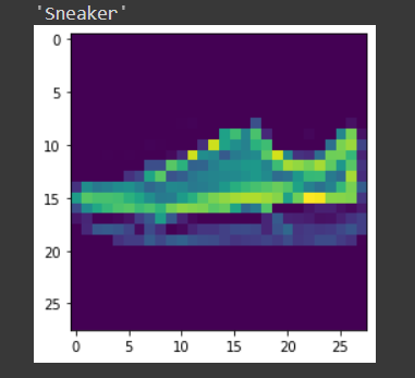
Step-10 Testing with a sample
The function defined for testing the model with a single image
def predict_image(img, model):
    # Convert to a batch of 1
    xb = img.unsqueeze(0)
    # Get predictions from model
    yb = model(xb)
    # Pick index with highest probability
    _, preds  = torch.max(yb, dim=1)
    # printing the image
    plt.imshow(img.squeeze( ))
    #returning the class label related to the image
    return train_set.classes[preds[0].item()]
img,label = test_set[9]
predict_image(img,model_scratch)
Conclusion
Here we had briefly discussed the main operations in a convolutional neural network and its architecture. A simple convolutional neural network model was also implemented to give a better idea of the practical use case. You can find the implemented code in my GitHub repo. Further, you can improve the performance of the implemented model by augmenting the dataset, using regularization techniques such as batch normalization and dropout in the fully connected layers of the architecture. Also, keep in mind that pre-trained CNN models are also available, which have been trained using large datasets. By using these state-of-the-art models, you will certainly achieve the best metric scores for a given problem.
References
- https://www.youtube.com/watch?v=EHuACSjijbI – Jovian
- https://www.youtube.com/watch?v=2-Ol7ZB0MmU&t=1503s-A friendly introduction to Convolutional Neural Networks and Image Recognition
About the Author
My name is Adwait Dathan, currently pursuing my master’s in Artificial Intelligence and Data Science. Feel free to connect with me through Linkedin.


