

This article is the second in a multipart series to showcase the power and expressibility of FlinkSQL applied to market data. In case you missed it, part I starts with a simple case of calculating streaming VWAP. Code and data for this series are available on github.
Speed matters in financial markets. Whether the goal is to maximize alpha or minimize exposure, financial technologists invest heavily in having the most up-to-date insights on the state of the market and where it is going. Event-driven and streaming architectures enable complex processing on market events as they happen, making them a natural fit for financial market applications.
Flink SQL is a data processing language that enables rapid prototyping and development of event-driven and streaming applications. Flink SQL combines the performance and scalability of Apache Flink, a popular distributed streaming platform, with the simplicity and accessibility of SQL. With Flink SQL, business analysts, developers, and quants alike can quickly build a streaming pipeline to perform complex data analytics in real time.
In this article, we will be using synthetic market data generated by an agent-based model (ABM) developed by Simudyne. Rather than a top-down approach, ABMs model autonomous actors (or agents) within a complex system — for example, different kinds of buyers and sellers in financial markets. These interactions are captured and the resulting synthetic data sets can be analysed for a number of applications, such as training models to detect emergent fraudulent behavior, or exploring “what-if” scenarios for risk management. ABM generated synthetic data can be useful in situations where historical data is insufficient or unavailable.
Intraday VaR
Value-at-Risk (VaR) is a widely used metric in risk management. It helps identify risk exposures, informs pre-trade decisions, and is reported to regulators for stress testing. VaR expresses risk as a monetary amount indicating the worst possible future loss on an asset, for a given confidence level and time horizon. For example, a 1-day 99% VaR of $10 on AAPL says that 99 times out of 100, a single share of AAPL won’t lose more than $10 the next day.
A common way to calculate VaR for equities is to take historical end-of-day returns (daily closing price changes for, say, the last 500 trading days) and treat them as a distribution of possible future returns. The VaR is the worst daily return at the 99th percentile (or the 5th worst return out of 500 days), multiplied by the current asset value. Assuming returns follow a normal distribution, another way to calculate VaR is to multiply the standard deviation by the z-score corresponding to the desired confidence interval which in our case is -2.58 for the 99% confidence interval left of the mean. The resulting figure is added to the average return, then multiplied by the current asset value to arrive at the VaR.
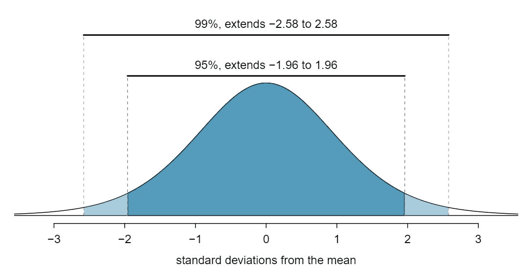
Image Source: https://spot.pcc.edu/~evega/ConfidenceIntervals.html
In most market risk applications, the VaR formula is based on end-of-day pricing and calculated daily in batches. This practice was prevalent in risk management ever since JP Morgan invented VaR in the 1980s. Since then, researchers have proposed methods for for calculating intraday VaR [1], driven by the evolving structure and dynamics of modern markets:
Over the last several years the speed of trading has been constantly increasing. Day-trading, once the exclusive territory of floor-traders is now available to all investors. “High frequency finance hedge funds” have emerged as a new and successful category of hedge funds. Consequently, risk management is now obliged to keep pace with the market. For day traders, market makers or other very active agents on the market, risk should be evaluated on shorter than daily time intervals since the horizon of their investments is generally less than a day.
Herein we explore how to calculate Intraday VaR (IVaR) from a real-time stream of tick data using streaming SQL. Specifically, we will calculate the 99% IVaR for every second based on the preceding 5 minutes of pricing data. For this exercise, we will be using synthetic market data generated by Simudyne. They have provided us with Level 1 tick data in CSV format for a fictional security (“SIMUl”):
time,sym,best_bid_prc,best_bid_vol,tot_bid_vol,num,sym,best_ask_prc,best_ask_vol,tot_ask_vol,num
2020-10-22 08:00:00.000,SIMUl,149.34,2501,17180,1,SIMUl,150.26,2501,17026,1
2020-10-22 08:00:01.020,SIMUl,149.34,2901,17580,2,SIMUl,150.26,2501,17026,1
2020-10-22 08:00:02.980,SIMUl,149.36,3981,21561,1,SIMUl,150.26,2501,17026,1
2020-10-22 08:00:05.000,SIMUl,149.36,3981,21561,1,SIMUl,149.86,2300,19326,1
2020-10-22 08:00:05.460,SIMUl,149.36,3981,21561,1,SIMUl,149.86,6279,23305,2
2020-10-22 08:00:05.580,SIMUl,149.36,3981,21561,1,SIMUl,149.86,6279,23305,2
2020-10-22 08:00:06.680,SIMUl,149.36,3981,21561,1,SIMUl,149.86,6279,23305,2
2020-10-22 08:00:07.140,SIMUl,149.74,582,22143,1,SIMUl,149.86,6279,23305,2
2020-10-22 08:00:07.600,SIMUl,149.74,582,22143,1,SIMUl,149.86,2044,19070,1
2020-10-22 08:00:08.540,SIMUl,149.74,582,22143,1,SIMUl,149.86,2044,19070,1
Level 1 tick data conveys the best bid price and best ask price in the security’s trading book for a given instant in time. We primarily care about the symbol and timestamp, as well as the market mid price, which we can take by averaging the best bid and ask prices. In order for Flink SQL to process this data, we first declare a streaming table through the following statement:
CREATE TABLE l1 (
    event_time     TIMESTAMP(3),
    symbol         STRING,
    best_bid_prc   DOUBLE,
    best_bid_vol   INT,
    tot_bid_vol    INT,
    num            INT,
    sym2           STRING,
    best_ask_prc   DOUBLE,
    best_ask_vol   INT,
    tot_ask_vol    INT,
    num2           INT,
    WATERMARK FOR event_time AS event_time - INTERVAL '5' SECONDS
) WITH (
    'connector' = 'filesystem',
    'path' = '/path/to/varstream/data/l1_raw',
    'format' = 'csv'
) ;
Time-Series Sampling in Flink SQL
In order to calculate IVaR, we need the distribution of second-by-second returns (the percent change in mid price from the previous second) for the past 5 minutes. If we treat the L1 data as a time-series, we need to sample the mid-price at every second. One way to do this is by filling forward: the sampled mid price for each second is the last observed mid price prior to, or at, that second.
Instinctively, we could try to do this with a tumbling window, as we did in Part I for calculating VWAP. However, this method will not work. Consider the tumbling window query below:
    SELECT
        symbol,
        TUMBLE_START (event_time, INTERVAL '1' SECOND) AS start_time,
        TUMBLE_ROWTIME (event_time, INTERVAL '1' SECOND) AS row_time,
        LAST_VALUE (best_bid_prc) AS best_bid_prc,
        LAST_VALUE (best_ask_prc) AS best_ask_prc
    FROM
        l1
    GROUP BY
        TUMBLE (event_time, INTERVAL '1' SECOND), symbol
    LIMIT 20
Tumbling windows may result in gaps as shown below.
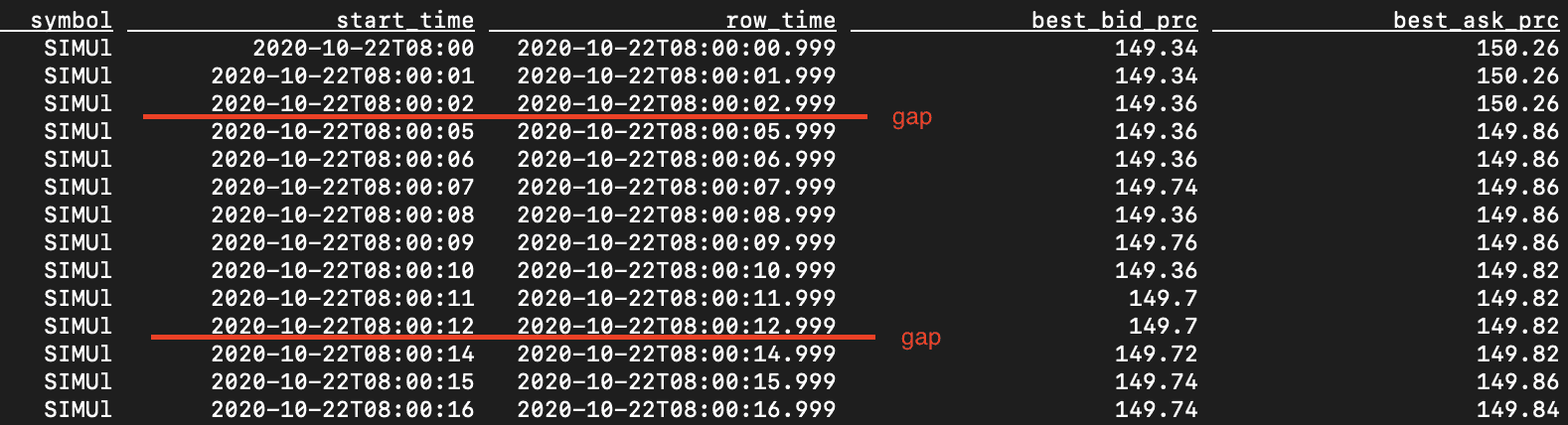
The query produced no rows for 8:00:03, 8:00:04, and 8:00:13. This is because in the source L1 data, there were no events during those second intervals. Potentially, one could fix this by using hopping windows instead, with a sufficient lookback period to ensure that there would have been an event observed during that period:
    SELECT
        symbol,
        HOP_START (event_time, INTERVAL '1' SECOND, INTERVAL '120' SECONDS) AS start_time,
        HOP_ROWTIME (event_time, INTERVAL '1' SECOND, INTERVAL '120' SECONDS) AS row_time,
        LAST_VALUE (best_bid_prc) AS best_bid_prc,
        LAST_VALUE (best_ask_prc) AS best_ask_prc
    FROM
        l1
    GROUP BY
        HOP (event_time, INTERVAL '1' SECOND, INTERVAL '120' SECONDS), symbol
    LIMIT 20
Unfortunately the above query will not run, since the LAST_VALUE function does not work with hopping windows as of time of writing. The Flink community is working on a fix (FLINK-20110). In the meantime, we present a workaround that does not rely on hopping windows nor a lookback period.
First we derive the effective time range (the start and end times) per row:
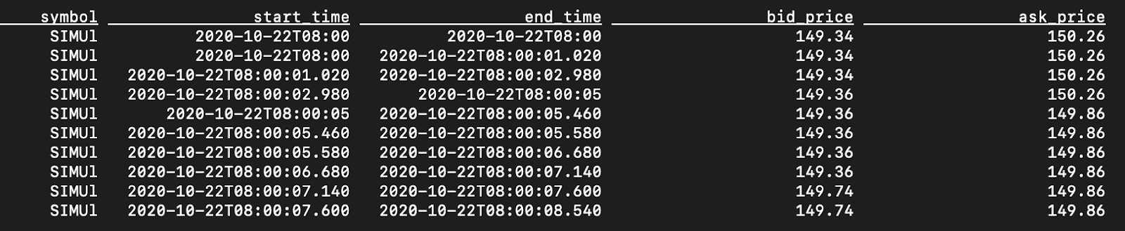
CREATE VIEW l1_times AS
    SELECT
        symbol,
        MIN (event_time) OVER w AS start_time,
        CAST (event_time AS TIMESTAMP) AS end_time,
        FIRST
        FIRST_VALUE (best_ask_prc) OVER w AS ask_price
    FROM l1
    WINDOW w AS (
        PARTITION BY symbol
        ORDER BY event_time
        ROWS BETWEEN 1 PRECEDING AND CURRENT ROW
    )
;
*Note the use of the MIN(event_time) instead of FIRST_VALUE(event_time)— currently, the FIRST_VALUE function does not support TIMESTAMP types.
This view streams the data while keeping the preceding row, emitting the field values of the preceding row, along with the current row’s event_time as the effective end time. A query against this view will yield the following, which shows that each row (except for the first) now has an inclusive start time and an exclusive end time.
In order to emit a row per second, we wrote a set of user defined table functions (UDTF). You can view the code here. The project has brief instructions on how to build the binary (a .jar file) and use it with Flink SQL. You will need to issue a CREATE FUNCTION statement to register each UDTF before using them in your queries:
CREATE FUNCTION fill_sample_per_day    AS 'varstream.FillSample$PerDayFunction'    LANGUAGE JAVA ;
CREATE FUNCTION fill_sample_per_hour   AS 'varstream.FillSample$PerHourFunction'   LANGUAGE JAVA ;
CREATE FUNCTION fill_sample_per_minute AS 'varstream.FillSample$PerMinuteFunction' LANGUAGE JAVA ;
CREATE FUNCTION fill_sample_per_second AS 'varstream.FillSample$PerSecondFunction' LANGUAGE JAVA ;
In queries, the UDTFs have the following syntax:
fill_sample_by_timeunit (start_time, end_time, frequency)
Where timeunit can be day, hour, minute, or second. The start and exclusive end times mark the effective time for each row, and frequency indicates how many times to sample the given day, hour, minute or second. So fill_sample_by_hour with a frequency of 6 will sample every 10 minutes (:00, :10, :20, :30, :40, and :50). Invoking fill_sample_by_minute with a frequency of 60 is functionally the same as fill_sample_by_second with a frequency of one. However, the by_second variant will perform better due to the internals of the UDTF implementation.
Now we can create a view that samples the stream every second. Note the use of INNER JOIN LATERAL TABLE, which ensures that the emitted rows will be controlled by the UDTF output:
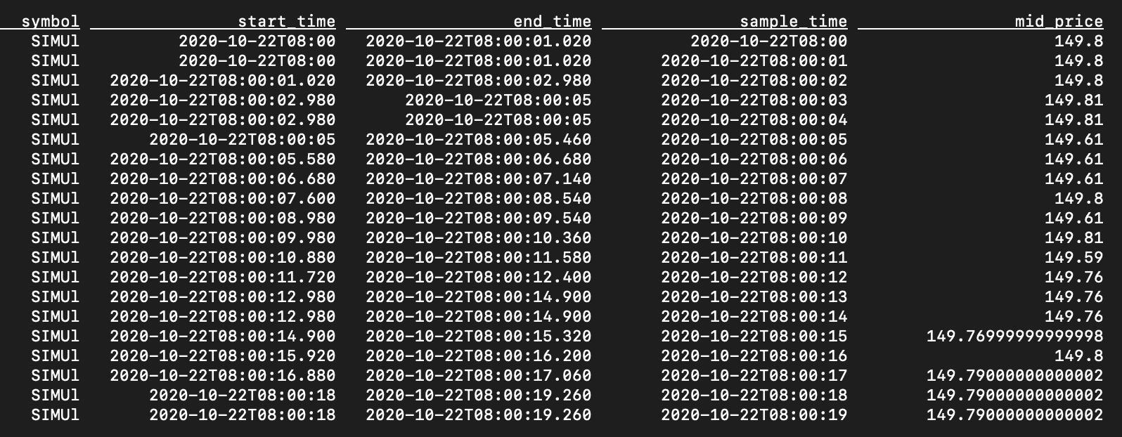
CREATE VIEW l1_sample AS
    SELECT
        symbol,
        start_time,
        end_time,
        sample_time,
        bid_price,
        ask_price,
        (bid_price + ask_price) / 2 AS mid_price
    FROM l1_times AS l1
    INNER JOIN LATERAL TABLE (fill_sample_per_minute (l1.start_time, l1.end_time, 60))
      AS T(sample_time) ON TRUE
;

SELECT symbol, start_time, end_time, sample_time, mid_price FROM l1_sample ;
Querying this view yields the following results.
Calculating Streaming Intraday VaR
Now that we have a time series sampled by second for the mid_price, we can start calculating the streaming IVaR. First, we need to calculate the returns for each second, which is simply the current price minus the previous price. To derive the previous price, we again use the OVER WINDOW syntax:
CREATE VIEW l1_sample_prev AS
    SELECT
        symbol,
        start_time,
        sample_time,
        mid_price,
        FIRST_VALUE (mid_price) OVER w AS prev_price
    FROM l1_sample
    WINDOW w AS (
        PARTITION BY symbol
        ORDER BY start_time
        ROWS BETWEEN 1 PRECEDING AND CURRENT ROW
    )
;
To get the 99th percentile of returns, we calculate the returns (expressed as a percentage) over a lookback window of the last 300 rows, which amounts to 5 minutes since we are sampling every second. We also calculate the average return and the standard deviation over the same window.
CREATE VIEW l1_stddev AS
    SELECT
        symbol,
        start_time,
        sample_time,
        mid_price,
        (mid_price - prev_price) / prev_price              AS pct_return,
        AVG (mid_price)                                    OVER lookback AS avg_price,
        AVG ((mid_price - prev_price) / prev_price)        OVER lookback AS avg_return,
        STDDEV_POP ((mid_price - prev_price) / prev_price) OVER lookback AS stddev_return
    FROM l1_sample_prev
    WINDOW lookback AS (
        PARTITION BY symbol
        ORDER BY start_time
        ROWS BETWEEN 300 PRECEDING AND CURRENT ROW
    )
;
With this information, we can derive the 99th percentile worst return by taking the product of the standard deviation and the Z-score of -2.58 and adding that figure to the average return. This is shown as var99_return below. The actual value at risk is the current mid price multiplied by var99_return. In the query below, we prefer to show the 99% worst possible future price of the asset, so we multiply the current price (mid_price) by 1 + var99_return.
CREATE VIEW l1_var99 AS
    SELECT
        *,
        avg_return - 2.58 * stddev_return AS var99_return,
        mid_price * (1 + (avg_return - 2.58 * stddev_return)) AS var99_price
    FROM
       l1_stddev
;

SELECT symbol, sample_time, mid_price, var99_price FROM l1_var99
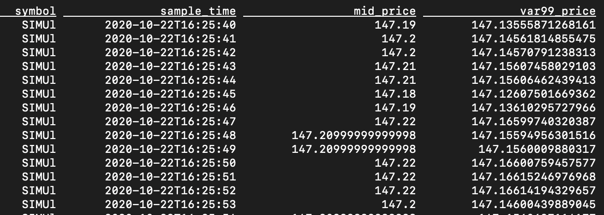
Conclusion
With high-frequency trading and mini flash crashes becoming more commonplace [2], understanding intraday market risk can be beneficial as is understanding one’s intraday exposure, particularly when using high-frequency algorithms. Fortunately, with a modern streaming platform like Flink, and an easy to use stream programming language like Flink SQL, we can quickly build robust pipelines to calculate intraday risk measures as market data arrives in real-time.
We hope this series will encourage you to try Flink SQL for streaming market data applications. For the next installment, we will show you how to try these examples using the upcoming version of Cloudera SQL Stream Builder, part of Cloudera Streaming Analytics version 1.4.
Thanks to Tim Spann, Felicity Liu, Jiyan Babaie-Harmon, Roger Teoh, Justin Lyon, and Richard Harmon for their contributions to this effort.
Citations
[1] Dionne, Georges and Duchesne, Pierre and Pacurar, Maria, Intraday Value at Risk (Ivar) Using Tick-by-Tick Data with Application to the Toronto Stock Exchange (December 13, 2005). Available at SSRN: https://ssrn.com/abstract=868594 or http://dx.doi.org/10.2139/ssrn.868594
[2] Bayraktar, Erhan and Munk, Alexander, Mini-Flash Crashes, Model Risk, and Optimal Execution (May 27, 2017). Available at SSRN: https://ssrn.com/abstract=2975769 or http://dx.doi.org/10.2139/ssrn.2975769
Editor's Choice