Measuring Validity and Reliability of Human Ratings
by MICHAEL QUINN, JEREMY MILES, KA WONG
As data scientists, we often encounter situations in which human judgment provides the ground truth. But humans often disagree, and groups of humans may disagree with each other systematically (say, experts versus laypeople). Even after we account for disagreement, human ratings may not measure exactly what we want to measure. How do we think about the quality of human ratings, and how do we quantify our understanding is the subject of this post.
Overview
Human-labeled data is ubiquitous in business and science, and platforms for obtaining data from people have become increasingly common. Considering this, it is important for data scientists to be able to assess the quality of the data generated by these systems: human judgements are noisy and are often applied to questions where answers might be subjective or rely on contextual knowledge. This post describes a generic framework for understanding the quality of human-labeled data, based around the concepts of reliability and validity. It then goes on to show how a new framework called cross-replication reliability (xRR) implements these concepts and how several different analytical techniques implement this framework.While human-labeled data is critical to many important applications, it also brings many challenges. Humans are fallible, and many factors can affect the kinds of judgments we collect. Along with the people completing the task, this includes the types of concepts that we’re measuring, the types of questions that we’re asking about these questions and the types of labeling tools provided to assign labels. For example, we’re often confronted by the fact that there’s simply no objective truth when assigning a label. How funny was that joke? How beautiful is that song? Was the dress blue or white? Although some of these tensions can never be fully resolved, we can make some progress towards answering harder questions by getting answers from many people.
Do these images depict a guitar?

Concepts for Measurement: Validity and Reliability
Archeological evidence suggests that people have been counting for at least 50,000 years, and we have pre-historical evidence for formal systems of measurement. If you wanted to know the size of a pyramid, you took a stick of known length, and you counted how many sticks you would need to reach from one side to the other. And for thousands of years, measurement was as simple as this. It was a process of adding units of something together and counting how many there were, to assess the magnitude of a physical quantity . The same procedure was just as valid for weight, volume, length, ticks of a clock, and most other measurements people cared about.The modern understanding of measurement wouldn’t be formally established until the end of the 18th century, with the creation of the science of Metrology. More formal systems of measurement began to be applied to ever more abstract concepts. For example, beginning in the early 20th century,
- researchers in social science and related areas were also thinking about measuring things like human ability and aptitude for different occupations
- sociologists tried to measure industrialization of different countries and social class
- political scientists studied political affiliation
- more recently, there have been efforts to take on much more subjective questions, like finding the world’s funniest joke
Reliability and validity: Definitions and measurement
Two fundamental concepts emerged from this research: reliability and validity.- A measure of an attribute is reliable if it is consistent, i.e., we get similar answers if we measure under similar conditions.
- A measure’s validity shows the extent to which variation in an attribute causes variations in a measurement.
For any procedure, reliability is necessary for high-quality data but not sufficient. A measure that is not reliable is not measuring anything particularly well, but a reliable measurement is only a good measure of something, not necessarily the right thing. This is where validity comes in. When measuring an attribute, we must assume that the thing we are trying to measure exists, and then validity tells us if we’re actually measuring it.
To help ground these terms, imagine you have a bathroom scale. While a measurement like weight seems to be pretty concrete, a variety of factors can introduce uncertainty about the “true value” that you’re measuring. For example, your weight fluctuates throughout the day, measurements are subject to lots of factors like whether or not you’re wearing clothes and we are not guaranteed to be using a perfect scale every time. Because of this, we might want to understand the reliability and validity of our approach to weighing ourselves.
If the scale gives the same measurement of your weight each time, it is said to have high reliability. But even if the scale fluctuates a lot, we can improve our measurement by repeating the same process multiple times under similar conditions. For example, you could weigh yourself multiple times in succession, and then take the average of these weights to improve the reliability of your measurement.
How else could you understand the quality of your scale? Well, you could weigh yourself at home before going to the doctor’s office and weighing yourself there. If you find out that your home scale is off by 5 lbs, then it has less validity than a more accurate scale. Similarly, you might also discover that your seemingly valid scale can have lots of variation every time you step on it. It can be accurate on average, but it is inconsistent. Reliability sets the upper bound on your validity, and you cannot measure something validly if you cannot measure it reliably.
Last but not least, if we think we are measuring height when people stand on the bathroom scales, multiple measurements will increase the reliability of the measure, but it is measuring the wrong thing: our measurement will never have high validity, even if height and weight are correlated. In this case, the scale is not measuring the construct that interests us.
Measurement challenges
Assessing reliability is essentially a process of data collection and analysis. To do this, we collect multiple measurements for each unit of observation, and we determine if these measurements are closely related. If the measures are sufficiently closely related, we can say that we have a reliable measurement instrument. If they are not closely related (for example, there may be considerable noise in the measures) we cannot say that we have a reliable measurement instrument.Assessing validity is equally important but often more challenging. To determine if our instrument is valid, we need to assess the degree to which it is giving us the right answers. For that, ideally we need data that tells us the underlying truth. We call this a gold standard or simply golden data. Of course, this golden data must also be reliable. Sometimes, obtaining gold standard data can be expensive and difficult; sometimes it is impossible to obtain good golden data, and we need to find a proxy that is close enough.
The fact that reliability and validity are so connected is key to the points we are highlighting today and the methods that we will be expanding. Measurements of reliability are critical when looking at human-labeled data, but they need to be complemented when possible by measurements of validity. The reverse relationship is also true. Measurements of validity probably shouldn’t be used in isolation. They should usually include their own measurements of reliability.
Non-parametric approaches to measuring reliability
To better understand the quality of the data in our tooling experiment, we need measurements of reliability and validity. We’ll start with the former by focusing on inter-rater reliability. From there, we will move towards a measurement of validity: our cross-replication reliability (xRR) framework.For those interested, these next sections that build to xRR closely follow the Wong, Paritosh and Arroyo paper that originally introduced all of this. We highly recommend you read that as well.
Cohen’s Kappa
Kappa was introduced in a paper by Jacob Cohen in 1960. Cohen was interested in the types of data collected in clinical and social psychology where a series of judges would categorize subjects into a strictly defined taxonomy. This type of data might appear when multiple psychiatrists make diagnoses on patients, or in studying various “leadership categories.” We can think of binary labels, like the images of guitars we discussed in the introduction, the same way. To answer the question “does this image contain a guitar?” There are two possible categories for someone to select: Yes, contains guitar, and No, does not contain guitar.At the time of Cohen’s writing, the most common approach was to compute what we now call “raw agreement,” the proportion of answers in the same category divided by the total number of responses. Cohen noted that this is often very misleading. Even when two independent people are labeling randomly, the probability of chance agreement remains quite high. This comes from the joint probability identities.$$
\Pr(X=x \cap Y = y) = \Pr(X = x) \times \Pr(Y = y)
$$To put some numbers behind this, two people flipping unbiased coins to determine the answer to the question of whether there is a guitar in the image will agree about 50% of the time, and the percentage of times that they agree increases as the distribution of answers moves away from 50:50. Imagine that they are each rolling a die, saying “Yes, guitar” if the die rolls a 6, and “No guitar” if the die does not roll a 6. The raw agreement will be (⅚ * ⅚ + ⅙ * ⅙) = 72%. If they roll two dice and apply a label if the dice rolls sum to 12 they will agree 85% of the time, purely by chance. Both people are behaving randomly, and not even looking at the images.
To help account for this expected level of agreement, Cohen proposed a measurement that could be applied when the following, relatively weak, conditions were met:
- The assessed units are independent
- Two people applying labels operated independently
- Categories are “independent, mutually exclusive and exhaustive”
\kappa = \frac{p_0-p_e}{1-p_e} = 1 - \frac{1-p_o}{1-p_e}
$$Where
- $p_o$ is the observed agreement between the people applying labels, i.e., the number of items where they agreed over the total number of items
- $p_e$ is the expected or chance agreement between our two labelers, which is derived from the number of times that each person labeled an item a particular category
p_e = \frac{1}{N^2} \sum_k n_{k1}n_{k2}
$$where $n_{k1}$ is the number of times the first person predicted category $k$, and $n_{k2}$ is the number of times the second person predicted this category.
Beyond Kappa, other types of outcomes
Kappa is traditionally computed on nominal outcomes, but many modern extensions have been developed to handle different outcome types. We will follow the example of Janson and Olsson, and start from this generalized definition of the metric, which they call iota. It starts from the same place as kappa above, as one minus the observed disagreement over the expected disagreement.$$\iota = 1 - \frac{d_o}{d_e}
$$The numerator, observed disagreement, is defined as the average-pairwise disagreement for labels within each item. Here it is:$$
d_o = \left[n {b \choose 2} \right]^{-1} \sum_{r < s} \sum_i^n D(x_{ri}, x_{si})
$$where
- $n$ is the total number of items
- $b$ is the number of people providing labels for each item
- $r$ and $s$ are indices for people providing labels
While the denominator, expected disagreement, can be computed by computing the average disagreement of all possible pairs, not just those within each item.$$
d_o = \left[n^2 {b \choose 2} \right]^{-1} \sum_{r < s} \sum_i^n \sum_j^n D(x_{ri}, x_{sj})
$$ In both cases, the key is to define a measurement of disagreement $D()$, a.k.a difference functions:
d_o = \left[n^2 {b \choose 2} \right]^{-1} \sum_{r < s} \sum_i^n \sum_j^n D(x_{ri}, x_{sj})
$$ In both cases, the key is to define a measurement of disagreement $D()$, a.k.a difference functions:
- Disagreement among continuous values can be measured using squared differences
- Nominal disagreement is acceptable for binary and other data types, i.e., we agree if the labels are the same for two items and disagree otherwise
- disagreement should be non-negative
- disagreement between a value and itself is alway zero
Measuring validity with xRR
While reliability measurements, like those discussed in the previous section, are useful for investigating the quality of human-labeled data, they are not sufficient for answering questions related to validity. In particular, human labelers can agree on an answer that is incorrect, and as we noted, a variety of other factors can influence the value of reliability that we observe. To help mitigate this, measurements of reliability are often paired with measurements of rater accuracy on golden data, i.e., datasets where we know the correct answer.Unfortunately, often the best golden data that we can obtain comes from experts. Experts are humans, and hence we have the same set of limitations we see when collecting any human-labeled data set:
- Items in golden datasets can be subjective, ambiguous or contextual
- The concept that we’re labeling is unknowable at one point in time or changes over time
- People make mistakes
Moreover, we face many cases where there simply isn’t a correct answer for a question. This ambiguity highlights something fundamental about the concept we are trying to measure. For example, do these images contain guitars?
Two different ways of looking at a seemingly simple concept, images of guitars
 |
| From Flick User Brickset (licensed under CC 2.0) and The Guitar Player (c. 1672) by Johannes Vermeer |
If experts disagree about whether a photograph of a Lego figure holding a Lego guitar contains a guitar, perhaps this is a sign that the construct we are trying to measure is not clearly defined in the first instance. Moreover, if a painting of a guitar from 1632 no longer looks like a modern guitar, we clearly have a concept that is mutable over time. In both cases, a somewhat concrete concept, like a guitar, becomes much more ambiguous when applied to particular cases, like legos and paintings from 1672. Since these problems cannot be simply wished away, we have to tackle the problem from a different angle. Doing so, we will introduce cross-replication reliability, or xRR.
Key concepts
Let’s take a step back. In the section above, we discussed the idea of inter-rater reliability, which we measured using Cohen’s kappa and other similar metrics. Regardless of the specific form of the metric, we are always comparing the labels of one person to another or to a pool of other people. In the xRR framework, we start thinking about using multiple pools. We have many different options for defining a pool:- We could randomly assign people to two groups during an experiment
- We could form different groups of people based on geography, demographics, etc.
- We might change something about our labeling process and are interested in comparing labels in the new process to labels in the old process
- We could compare a group of experts to a broader general population
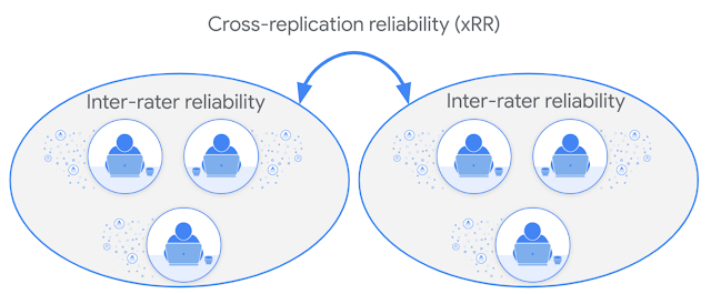
When you have two different groups labeling data, inter-rater reliability measures the within-group consistency, while cross-replication reliability (xRR) measures consistency between the groups. When one of the groups consists of experts, xRR functions as a measurement of validity.
Understanding xRR in light of golden data
Measuring something without a pre-existing gold standard is quite difficult, even when assessing physical quantities like length, or weight. To solve this problem, we follow the philosopher Karl Popper, who defined objectivity as intersubjectivity. If we measure a quantity using two methods, and these methods agree, we have greater belief that we have a valid measurement.For example, physicists want to measure the speed of light. There are many options to do this, and we’ll highlight two:
- one method is to use the apparent motion of Jupiter’s moon (Io)
- another method is to use laser interferometry
Things are a little different in our field, since we do not expect perfect agreement, even among experts. We need to update our metrics to be able to account for this disagreement. To do this, we need to set a measurement of reliability for our experts, as this sets the upper limit on validity. With that, we can get a measurement of validity by assessing agreement: we ask how much agreement we would expect to have, given the inherent lack of reliability in our data. This is xRR.
Computing xRR
\kappa_x(X,Y) = 1 - \frac{d_o(X,Y)}{d_e(X,Y)}
$$Our measurement of xRR (cross kappa) compares the observed disagreement between two groups with the expected disagreement between groups. Like kappa, we define the numerator and denominator using a disagreement metric. Here’s the numerator, the observed disagreement across groups:$$
d_o(X,Y) = \frac{1}{n R S} \sum_{i=1}^n \sum_{r=1}^R \sum_{s=1}^S D(x_{ri}, y_{si})
$$We average disagreement over $n$ items, $R$ labels per item in the $X$ group and $S$ labels per item in the $Y$ group. This formula is derived by creating all pairs of labels for each per in each group, where both people provided a label for each item.
The formula for the denominator, the expected disagreement across groups, is $$
d_e(X,Y) =
\frac{1}{n^2 R S} \sum_{i=1}^n \sum_{j=1}^n \sum_{r=1}^R \sum_{s=1}^S D(x_{ri}, y_{sj})
$$The formula is quite similar to that of the numerator, with one addition. Instead of comparing pairs of labels across matching items, we compare pairs of ratings across all possible combinations of items.
As we mentioned with kappa above, the choice of disagreement metric is flexible.
- We can represent disagreement in continuous data using the square difference between two points
- We can represent disagreement in categorical data by comparing labels and counting how often pairs of labels are different
Here’s an example. Let’s start with a very simple case, we have four items, two groups, each of which has two people providing binary labels. We will use nominal agreement to compute xRR.

To get the observed disagreement, you create all possible within-item pairs between people in group one and group two, count the total disagreement and divide by the number of pairs.

Here, there are 16 pairs, and the observed disagreement is 0.25. In other words, on the two items that we have, raters from the first group disagree with raters from the other group one quarter of the time.To get expected agreement, the computation is similar, but we also create all pairs across all items. That gives us 64 comparisons instead of 16. Expanding out all of those combinations, we find that there is a 0.4375 rate of disagreement. Plugging these values into our formula gives us a cross kappa that is close to 0.43.
Normalized xRR
xRR gives us a measurement of similarity between the labels of individuals from two different groups for the same items. Since we usually collect multiple labels per item from each group, we can aggregate the ratings for an item from each group, say, by taking the mean or modal category. We have a way to use xRR measurements to compare these aggregated ratings. We call this normalized xRR. Here’s how we define it for the cross kappa metric.$$\mathrm{normalized\ }\kappa_x = \frac{\kappa_x(X,Y)}{\sqrt{IRR_X}\sqrt{IRR_Y}}
$$As described above, Normalized xRR is just xRR divided by the product of the square roots of the inter-rater reliability for each group, i.e., kappa.
This normalization is very similar to attenuation-corrected correlation. We can often treat this measurement as a correlation between the aggregated values of each group, or in general, think of it as a validity measurement for the aggregated ratings across pools. In other words, while xRR can be used as a measurement of how close a generalist's rating is to that of an expert, normalized xRR tells us how the aggregate of generalist labels correlates with the aggregate of expert labels.
Inference for non-parametric reliability and validity measurements
There are derivations for standard errors and confidence intervals for some non-parametric reliability metrics. For example, Fleiss, Cohen and Everitt provided formulas for Kappa and Weighted Kappa. But for more complicated metrics like xRR, our preference is to bootstrap when measuring uncertainty.
Parametric measurements
Thus far, we’ve been discussing non-parametric approaches to measuring reliability and validity, but in this section we’ll present an approach to get the same measurements from parametric models. There are many good reasons for doing this:- Models come with explicit assumptions, and these are worth investigating when thinking about our measurements
- We can be more flexible with the structure of the model to account for peculiarities in particular data generating processes
- The models that we’ll be using come with built-in measurements of uncertainty, making it much easier to do statistical inference on our measurements of reliability
- Models need to be fit, and fitting the types of models that we’ll be using is often much more computationally expensive than non-parametric measurements of reliability
- A model’s assumptions can be incorrect and misspecified models can lead to incorrect conclusions
Throughout, we’ll refer to our model-derived measurement of inter-rater reliability as the Intraclass Correlation Coefficient (ICC). To be fair, this will be a small abuse of terminology, especially as we move away from the most standard versions of this metric. Nonetheless, there is a robust literature around this type of measurement, and the term ICC, or small variations thereof, is used consistently.
The simplest case, continuous outcomes
To help motivate our understanding of ICC, we’ll start with the simplest case, where the labels are continuous scores over a sufficiently large enough range, say 0 to 100. Each item receives multiple labels, and each person labeling this data assesses multiple items. Consuming this data, we’ll often care about the mean of multiple labels. In this case, we could apply the model this data using the following:$$\begin{align*}
Y_i &\sim \mathcal{N}(\theta_i, \sigma^2) \\
\theta_i &= \mu + \eta_{i[j]} + \eta_{l[k]} \\
\eta_{i[j]} &\sim \mathcal{N}(0, \sigma_i^2) \\
\eta_{l[k]} &\sim \mathcal{N}(0, \sigma_l^2)
\end{align*}
$$There’s a lot of notation there, so we’ll go through it line-by-line.
- We treat each individual score $Y_i$ as a draw from a normally distributed random variable, with a single variance parameter $\sigma$
- The mean of this random variable comes from the linear predictor, $\theta_i$, which consists of
- a baseline average score for all items, $\mu$
- a latent value for each of the $j$ items in our dataset, $\eta_i$; here, the subscript $i$ refers to the item being labeled
- a bias for the $k$ labelers, $\eta_l$
- The two latent variables $\eta$ in our model come from normal distributions, each with its own variance parameters ($\sigma_i$ and $\sigma_l$)
- Each labeler only gives one score per item, but they can label many different items
- Each items has an underlying “true score” and deviations in the observed scores are the result of consistent labeler bias and random noise
- Speaking of labeler bias, this model assumes that raters respond to items in a consistent and additive fashion:
- When looking at jokes, some people will find all jokes really funny, while others will think that none of the jokes are funny
- The same follows for less subjective tasks; for example, different proofreaders might assess grammar with varying degrees of strictness
Note: In practice, we would also add some priors for the variance parameters in our model. We normally have lots of labelers and items in our dataset, and priors give a form of regularization that better handles cases where data might be sparse and makes the model less prone to overfitting.
We derive our measurement of data quality, ICC, from the variance parameters in the model.$$ICC = \frac{\sigma_i^2}{\sigma_i^2 + \sigma_l^2 + \sigma^2}
$$That is, the ICC is the ratio of the variance parameter for the “true score” of each item over the total variance in the model. This version of ICC is the same as a Variance Partition Coefficient (VPC), and it tells us how much variance in the model can be attributed to a particular model component. Values closer to 1 indicate higher data quality, while values closer to zero indicate lower data quality. In the most extreme case, each labeler would provide the exact same score for each item. We would observe no labeler bias or random noise. All of the variance in the model would be explained by differences in the true scores for the items, and our ICC would be equal to 1.
ICC as a reliability measure
Another way to interpret this value is to think of it as a correlation, as the name would imply. The ICC is the squared correlation between a single person’s label and a “true” label. Given that the expectation of a random rating by a random rater is equal to the true score for that item, we can derive it from aggregating the responses of an infinite number of people. Looked at another way, it is the correlation between a single persons’ score for an item and the average of scores from an infinite number of other people.That last part is a little weird. An infinite number of other people? While it may be a little abstract, this concept forms a key piece of Classical Test Theory (CTT), a foundation of psychometrics. The basis of CTT is the equation that looks like this$$
Y = T + e
$$Where
- $Y$ is the label for item $i$ given by person $j$,
- $T$ is the True Score for item $i$, i.e., expected value of labels from all people (see Borsboom, 2005)
- and $e$ is random error, with a mean of $0$
We can derive this by looking at the variances of the variables in our equation above. By definition, the covariance of $T$ and $e$ is zero, and therefore the variance of $y$ is given by:$$
\mathrm{var\ }Y= \mathrm{var\ }T + \mathrm{var\ }e
$$Thus $\mathrm{var\ }T$ is the proportion of variance in the measured variable $Y$ that is accounted for by True Score. This is equivalent to $R^2$ in a regression equation. That brings us back to the definition of ICC from before, as the correlation between one response and the aggregate over an infinite number of responses.$$
ICC = \frac{\mathrm{var\ }T}{\mathrm{var\ }T + \mathrm{var\ }e}
= \frac{\mathrm{var\ }T}{\mathrm{var\ }Y}
= \frac{\sigma_i^2}{\sigma_i^2 + \sigma_l^2 + \sigma^2}
$$Going back to the version of ICC defined above, our model’s version of the True Score is the latent parameter $\eta_i$, and $\mathrm{var\ }T$ is equal to the item-level variance $\sigma_i^2$. Variance is additive in the model in the preceding section, meaning that $\mathrm{var\ }Y$ is the sum of the three variance parameters in the model, i.e., the sigmas.
Note: Readers with a background in social science may have come across Coefficient (or Cronbach’s) alpha published in 1951; alpha is an alternative method of calculating the ICC.
Spearman-Brown prediction formula
In practice, we don’t usually consume labels as singletons. We instead collect multiple labels for the same item and generate aggregates, like the mean of multiple labels when they are continuous. We would also like to be able to say something about the reliability of these means along with the reliability of the individual scores, in the same way that normalized xRR can tell us about the validity of the aggregates.This is straightforward to work out, using the definition of reliability from above. We will combine k items together to create an aggregate score. Then, we can calculate the variance of the new score by applying the classic formula for linear combinations of variances. Applying the formulas from the previous section, and remembering that the true score correlation is one across tests while the error correlation is zero, we get $$
\mathrm{var\ }(k Y) = k^2 \mathrm{var\ }T + k\ \mathrm{var\ }e
$$We can use the definition of ICC from above, as a proportion of variances, to complete the derivation:$$
\begin{align*}
ICC(k) &= \frac{k^2 \mathrm{var\ }T}{k^2 \mathrm{var\ }T+k\ \mathrm{var\ }e}\\
&= \frac{k^2 \mathrm{var\ }T}{k^2 \mathrm{var\ }T+k(\mathrm{var\ }Y-\mathrm{var\ }T)}\\
&= \frac{k\ \mathrm{var\ }T}{k\ \mathrm{var\ }T + \mathrm{var\ }Y-\mathrm{var\ }T}
\end{align*}
$$We can use the definition of ICC from above, as a proportion of variances, to complete the derivation. Dividing the numerator and denominator by var(y), we get everything in terms of the ICC.$$
ICC(k)=\frac{k\ ICC}{k\ ICC+1-ICC} = \frac{k\ ICC}{(k - 1) ICC+1}
$$This is the Spearman-Brown prediction formula. It was developed and published independently in 1910 by Charles Spearman (who is remembered for his work on factor analysis, intelligence, and correlation) and William Brown (who is not remembered much any more). Both published articles in the same volume of the British Journal of Psychology.
One particularly useful application of this formula is task design, and we treat $k$ as the proportional change in the number of people applying labels to each item. For example, if we start with two people assessing each item, and we increase it to four per item, then we have doubled the number of labels per item, and therefore $k = 2$. Once we understand the reliability of an individual response, we can establish plans to collect a certain number of labels for a task until we reach a predetermined threshold.
- insufficient labels means that our data is possibly insufficiently reliable
- an excessive number of labels means that we may have wasted resources since we could have obtained results that were almost as good with a smaller number of labels
Different outcome types
The simplest model we can use to compute ICC has continuous outcomes, but the model can be extended to handle other outcome types, like binary (0, 1) values. This gives us a measurement that is often quite similar to Cohen’s kappa from above. Here is our updated model.$$\begin{align*}
Y_i &\sim \mathrm{Bernoulli}(p_i) \\
p_i &= \mathrm{logit}^{-1}(\theta_i) \\
\theta_i &= \mu + \eta_{i[j]} + \eta_{l[k]} \\
\eta_{i[j]} &\sim \mathcal{N}(0, \sigma_i^2) \\
\eta_{l[k]} &\sim \mathcal{N}(0, \sigma_l^2)
\end{align*}
$$This model is quite similar to what we already discussed, but
- We now treat $Y_i$ as a draw from a Bernoulli distribution, taking either values of 0 or 1
- The probability of an outcome $p_i$ is based on the inverse logit of the same linear predictor as the previous model $\theta_i$
ICC = \frac{\sigma_i^2}{\sigma_i^2 + \sigma_l^2 + \pi^2/3}
$$This also means that our understanding of the ICC changes somewhat as well. We are now talking about proportions of variances on the latent scale of the model. This is more than a theoretical quibble. Using this implied variance for the ICC produces values that are somewhat larger than other approaches. The actual variance in the outcome, which is determined by the number of positive and negative cases, is ignored when we always use $\pi^2/3$. This also means that our extreme example from above, where all labelers perfectly agree, cannot produce an ICC of one.
Some words of caution on interpreting reliability metrics
We are often asked about acceptable or unacceptable values for the ICC, i.e., how do I know when my ICC is good enough? Unfortunately, this is not a question that can be answered easily, as it is often tied to the labeling task at hand. More concrete tasks might require a higher acceptable threshold for ICC, which might be closer to the criteria set by Landis and Koch, where anything above 0.6 is considered acceptable. In practice, with more diverse and subjective tasks, we often see acceptable ICC values that are much lower.To further complicate matters, many other factors can influence these metrics. Notably:
- High class imbalance decreases reliability metrics, especially those that are chance-corrected, like Kappa
- People will naturally agree less on more subjective questions. Even seemingly objective questions can be ambiguous when applied to certain items (is the dress blue or white?)
- The types of people labeling the data might influence reliability; e.g., many tasks have a strong cultural component
ICC_{l} = \frac{\sigma_l^2}{\sigma_i^2 + \sigma_l^2 + \sigma^2}
$$Following the VPC interpretation of ICC from above, this metric tells us how much variance in the model is explained by patterns in responses from particular raters. We want this to be as low as possible. At the extreme, each labeler could give the exact same score to all of the items they see. In that case, all of the model variance would be determined by this special score chosen by each labeler. The Labeler ICC would be equal to one while the (standard) ICC would be zero.While we can’t always give a specific acceptable threshold for ICC, we would consider human-labeled data unacceptable if the Labeler ICC exceeded the ICC.
Normalized xCC: A parametric measurement of Normalized xRR
Just as we used a model to produce parametric versions of reliability metrics, we can also use a model to generate a measurement of xRR. As before, we’ll begin with the simplest case, treating the outcome variable as continuous. As before, note that this simpler model can be extended to handle many different outcome types.We can model this as follows:$$
\begin{align*}
Y_i &\sim \mathcal{N}(\theta_i, \sigma^2) \\
\theta_i &= \mu_s + \eta_{i[js]} + \eta_{l[ks]} \\
\eta_{i[j0]}, \eta_{i[j1]} &\sim \mathcal{N}(\mathbf{0}, \mathbf{\Sigma}_i) \\
\mathbf{\Sigma}_i &= \mathbf{S R S} \\
\mathbf{S} &=
\begin{bmatrix}
\sigma_{i0} & 0 \\
0 & \sigma_{i1}
\end{bmatrix}\\
\mathbf{R} &=
\begin{bmatrix}
1 & \rho \\
\rho & 1
\end{bmatrix}\\
\eta_{l[k]} &\sim \mathcal{N}(0, \sigma_{l[s]}^2)
\end{align*}
$$As before, we’ll go through it line-by-line.
- As in the original model, each of the $i$ scores $Y$ is assumed to be a draw from a normally distributed random variable, with a single variance parameter $\sigma$
- The mean of this random variable comes from the linear predictor, $\theta$, which consists of
- a baseline average score for all items, $\mu$.
- We have $j$ total items in the data set
- The baseline can differ across each of our user interface studies, which we’ll call $s$
- a latent value for each of the items in our dataset, $\eta_i$
- Because the same items are labeled by two different groups, we differentiate them using $s$
- This differs across studies but remains correlated. The correlation is determined by the parameter $\rho$
- The variance within studies can differ as well, which is why we now have two values for $\sigma_i$
- a bias for the labelers, $\eta_l$
- We compute $k$ of these bias values, mapping to the number of unique people providing labels
- The degree of bias among the labelers can also differ between the studies, giving us multiple values for $\sigma_l$
- The latent variables $\eta$ in our model come from normal distributions, each with their own variance parameters ($\Sigma$ and $\sigma_l$).
- An item is labeled in multiple studies ($s$)
- Different groups of people participate in each study
- Most of our parameters in our model have values for each of these studies
- And the biggest change is that the there is a relationship between the underlying latent values for items across studies, as capture in the correlation parameter $\rho$
The value of this $\rho$ parameter is ultimately what we want. One way to interpret this parameter is that it tells us how correlated mean measurements are across studies, accounting for rater bias. In that sense, it can be treated similarly to normalized xRR, which we discussed above. As ICC is the parametric measurement of reliability, we can call this $\rho$ parameter "normalized xCC".
Getting “unnormalized” xCC from the model
Our parametric model produces a value that has a similar interpretation to normalized xRR. We can compute the original xCC (our metric for xRR) using this identity from Wong, Paritosh and Arroyo. $$\mathrm{xCC} = \rho \sqrt{ICC_0} \sqrt{ICC_1}
$$ where each of the ICC values are computed using parameters that match a particular group within our study, e.g., group zero might be the generalists while group one is the experts. For example, to get the ICC for items in the first study, mapped to index zero, we would compute the following:$$
ICC_0 = \frac{\sigma_{i0}^2}{\sigma_{i0}^2 + \sigma_{l0}^2 + \sigma^2}
$$The ICC is computed using variance parameters mapping to that study. We follow the same approach to get ICC_1.How do we understand this ICC? Other approaches to computing an ICC, like that of Johnson or Stoffel, Nakagawa and Schielzeth, compute this metric over all the groups together. Here, we are explicitly choosing only a subset. In practice, we see that the ICC computed this way is almost always equal to the version derived exclusively from the relevant slice of the data, regardless of the value of $\rho$.
A case study: Measuring impact of changes to labeling tools
As a concrete example, let's analyze data that was labeled for policy enforcement: making sure that the ads we show are safe. When labeling this sort of data, people usually answer the following question: is this item (usually an ad) in violation of a particular Google policy?Within this study, we have one expert group of people providing labels, which we’ll call the reference group. Collecting data exclusively from this group isn’t possible, since we don’t have enough experts to handle the volume of labels that we need. But we would prefer it if the data we collect was as close as possible to expert quality. We also have two generalist groups of people providing labels, each using a different set of tools. For the purpose of this example, we can assume that the subjects were randomized into the two groups which we’ll call control and treatment. We recently updated the set of labeling tools that we made generally available, and we want to know if these changes positively impact the quality of data we received from the general group of people providing labels. For comparison, the control group uses the original tools.
A sample of a couple rows of this data can be found below.

In this dataset, it’s important to point out that:
- Hundreds of ads were labeled for this study
- Each ad was labeled multiple times, giving us thousands of labels for each group
- There is a large and diverse set of labelers in each group who might come from different countries, speak different languages, be different ages
- Everyone provided multiple labels
- Each item is labeled multiple times
- No person labeled the same item twice
To start, it helps to look at the basic distribution of responses in our dataset. Did the groups agree on the rate that an item violated a policy? In what follows, assume we have a large number of items and people, so that the measures have little statistical uncertainty.

Naively looking at these rates, we would believe that our control group is over-flagging items as policy violations. The treatment group seems to be more in line with the reference group, but it’s hard to say if the difference in flagging rates is meaningful, even if it is statistically significant.
Of course, rates will often miss several key details that we should care about:
- Do we see agreement or disagreement in the labelers' responses within each group?
- Are the items being flagged as policy violating by treatment and control similar to those being flagged by our expert group?
- Does the change in tooling, our treatment effect, lead to improvement in these areas?
Reliability measurements in our policy study
The first step in understanding the impact of the tooling change is to look at measurements in reliability. The following table shows kappa, a non-parametric measurement, and ICC, our parametric measurement, across different groups of people involved in our tooling study.

As discussed, concrete benchmarks for reliability are hard, but all three measurements above can be considered quite high. At the very least, they all exceed the Landis and Koch threshold for “high agreement.”
But that leads to a somewhat counterintuitive result. We previously saw that our control group might have been over-flagging items as policy violations, and now, we see that the reliability of the control group is higher than that of our experts. This is curious, to say the least, since one would naively believe that experts deliver the most reliable data for this task. The change in tooling also led to a considerable decrease in reliability in our treatment group. A lot of factors may have contributed to this. Perhaps the simple fact that the tools were new contributed.
Nonetheless, an outcome like this isn’t necessarily a negative one for our experiment. Even though the control group had more consistency than the treatment group, we still don’t know if they were validly applying policy labels.
xCC in our study
Now that we have looked at reliability, what does xCC tell us about the shifts in quality observed in our tooling study? We compute xCC for both treatment and control against the reference group of experts. The difference of xCCs between treatment and control tell us which of the two groups is closer to the experts. We also do the same comparison but with normalized xCC. This gives us the following charts and table.

While the size of the xCC difference is small, it is still most likely greater than zero. The fact that this difference is small is in part due to the fact that we also saw a lower reliability in the treatment group when compared to control. Meanwhile, the normalized xCC difference is definitely not small. In other words, a person using the new tooling is somewhat closer to the opinions of experts, but we also see that (perhaps more importantly) the aggregated opinion on items in the treatment group are much closer to those of experts. Either way, both metrics indicate that the change in tooling leads to labeling outcomes that better reflect the opinions of experts. This example illustrates important lessons for understanding the quality of human data, bringing us back to the concepts introduced in the beginning of the article. We want a measurement that is both reliable and valid. Within our tooling experiment, the control group appeared to be reliable, with very high values of kappa and ICC, but the over-flagging rates and xCC metrics show us that the control group’s measurement was less valid (when experts are the reference) than that of the treatment group. The shift in tooling ultimately had a positive effect.
Conclusion
We hope you’ve enjoyed this tour of these key measurement concepts and their application to human-labeled data. Throughout business and science, we use people to measure things that cannot be measured any other way. Once we take this step, we encounter a host of interesting challenges: people's judgments can be noisy and biased, and often the concept that we are measuring has no single objective value. Because of this, we have to establish additional frameworks to understand the quality of our metrics.In this blog post, we talked about two such approaches:
- Within a single group, measure a concept many times and assess the quality of that measurement using a reliability metric
- If you also have a pool of experts, you can also understand the validity of your measurement with a technique like xRR
References
- A coefficient of agreement for nominal scales (Cohen, Jacob. Educational and psychological measurement 20.1 (1960): 37-46)
- A Measure of Agreement for Interval or Nominal Multivariate Observations (Janson & Olsson, Educational and Psychological Measurement, 61(2), 277–289)
- Answering the call for a standard reliability measure for coding data (Hayes & Krippendorff. Communication methods and measures 1.1 (2007): 77-89)
- Computing Krippendorff's Alpha-Reliability (Krippendorff, 2011)
- Cross-replication Reliability - An Empirical Approach to Interpreting Inter-rater Reliability (Wong et al., ACL-IJCNLP 2021)
- Data Excellence: Better Data for Batter AI (Aroyo, L. NeurIPS 2020)
- Extension of Nakagawa & Schielzeth's R2GLMM to random slopes models (Johnson, Methods in ecology and evolution, 5(9), 944-946)
- krippendorffsalpha: An R Package For Measuring agreement Using Krippendorff’s Alpha coefficient (Hughes, arXiv:2103.12170 [stat.ME])
- Large sample standard errors of kappa and weighted kappa (Fleiss, et al., Psychological Bulletin, 72(5), 323–327.)
- Measuring the Mind: Conceptual Issues in Contemporary Psychometrics (Borsboom, D., 2005)
- Partitioning variation in multilevel models (Goldstein et al., Understanding statistics: statistical issues in psychology, education, and the social sciences, 1(4), 223-231)
- Pervasive Label Errors in Test Sets Destabilize Machine Learning Benchmarks (Northcutt, et al., arXiv:2103.14749 [stat.ML])
- rptR: Repeatability estimation and variance decomposition by generalized linear mixed‐effects models (Stoffel, et al., Methods in Ecology and Evolution 8.11 (2017): 1639-1644)
- The coefficient of determination R2 and intra-class correlation coefficient from generalized linear mixed-effects models revisited and expanded (Nakagawa, et al., J. R. Soc. Interface 14: 20170213)
- The Measurement of Observer Agreement for Categorical Data (Landis & Koch, Biometrics, 33(1), 159–174)
Comments
Post a Comment